Carlos Pestana Barros & Nicolas Peypoch
A Comparative Analysis of Productivity Change in Italian and Portuguese Airports
WP 006/2007/DE _________________________________________________________
António Afonso
Euler Testing Ricardo and Barro in the EU
WP 23/2008/DE/UECE _________________________________________________________
Department of Economics
WORKING PAPERS
ISSN Nº0874-4548
School of Economics and Management
Euler testing Ricardo and Barro in the EU
*
António Afonso**
Abstract
According to Keynesian economics wisdom, government debt has an effect on the economy since consumers see government debt as net wealth. However, according to the debt neutrality hypothesis of Ricardo (1817), popularised by Barro (1974), such effects would be absent. This paper’s results, obtained from Euler equation estimations using a panel data approach, indicate that it would be wise to reject the debt neutrality hypothesis for the EU and that higher government indebtedness could actually deter private consumption.
JEL classification: C23; E21; E62; H63
Keywords: debt neutrality; private consumption; EU; panel data
*
The opinions expressed herein are those of the author and do not necessarily reflect those of the ECB or the Eurosystem.
**
European Central Bank, Directorate General Economics, Kaiserstraße 29, D-60311 Frankfurt am Main, Germany, email: [email protected].
1 – Introduction
Government debt neutrality and the Ricardian Equivalence hypothesis have been one of the most debated issues of modern macroeconomics, and the subject of a large number of theoretical and empirical research papers. Under conventional macroeconomic analysis, government debt usually has an effect on the economy since consumers consider government debt as net wealth. Therefore, the bigger the stock of government debt the wealthier consumers feel and the more inclined they are to consume.
The key idea behind Ricardian Equivalence is that consumers are linked by intergenerational altruism, and also that they have a fairly good perception about the future taxes needed to repay the present increase in government debt. Consumer’s net wealth would be invariant between more debt today and more taxes tomorrow. By this reasoning, budget deficits would have no real effects and fiscal policy would be unable to change consumption, quite a different notion from the one sustained by Keynes. In a limit situation, when the government reduces taxes, consumers just save more, for instance placing money in time deposit accounts, in order to help pay the higher future taxes, and consumption remains unchanged.
This paper adds to the existing literature, by using a panel data approach for testing the debt neutrality hypothesis, via the response of private consumption EU countries. Moreover, the advantages of panel data methods, within the macro-panel setting, include the use of data for which the spans of individual time series data are insufficient for the study of many hypotheses of interest, such as the the issue of government debt neutrality in our case. The remainder of the paper is organised as follows: in section two, debt neutrality is briefly discussed; section three derives the Euler equation set up, resulting from the consumer’s inter-temporal optimisation problem; section four presents the empirical analysis for the EU; section five is a conclusion.
2 – Government debt neutrality
Barro’s (1974) paper definitely set a landmark and represented a turning point of the literature concerning the government debt issue. The necessary conditions for the Ricardian Equivalence to hold are clearly presented on that paper, namely the intergenerational solidarity model, with a theoretical set up inspired in the overlapping generations model of Samuelson (1958) and Diamond (1965).1 The link between generations is paramount to guarantee the debt neutrality result, one of the so-called five neutrality results of New Classical economics in Akerlof’s (2007) terminology.
Under certain conditions, it would be irrelevant how the deficits are financed, implying the assumption of the Ricardian Equivalence hypothesis, as stated already in the early XIX century by Ricardo (1817). In a simplified way, the main idea of the debt neutrality proposition dwells on the supposition that government debt and lump sum taxes are equivalent methods of financing a given amount of public expenses. Deficits merely postpone the future imposition of taxes. If consumers are rational, it becomes indifferent to pay 100 Euros of taxes today or tomorrow. In that sense, being irrelevant to the consumers the moment when taxes are paid, consumers do not change their consumption decisions after variations in the budget deficit. Therefore, one of the several implications of the theorem’s
1
validity is the result of debt neutrality, when the deficit is financed by government debt, that is, deficits do not influence real variables, and have no effects on aggregate demand.
For instance, Phelps (1982, pp. 379) considers that increases in the supply of government debt ends up creating its own demand, and it would not influence the demand for other assets. In other words, there would be a sort of “Say’s Law” for the deficits and the respective financing by government debt. Nevertheless, one must recognize that Ricardo was convinced that in practice it was quite relevant the method the government chooses to finance its expenses. This conviction of Ricardo led O’Driscoll (1977) to suggest that the Ricardian Equivalence Theorem should be called “Ricardian Nonequivalence Theorem.”2
Usually, the critics to the Ricardian Equivalence hypothesis focus on distortionary taxation, and intergenerational altruism and capital markets efficiency.3 For instance, Sims (1998) states in a vigorous way that the Ricardian Equivalence theorem is irrelevant for the reality economists try to understand and formalise, while Buiter (1985) holds that “neutrality of public debt and deficits is little more than a theoretical curiosum.” It should therefore be considered as an extreme situation since taxes are not lump-sum, some prices are not perfectly flexible, people do not live forever and many people do not have ascendants or descendants willing to help them financially.
The altruistic behaviour is also open to much criticism and discussion. The absence of intergenerational transfers may for instance be the result of divergent preferences among household members.4 Also, the opposition between finite horizons and infinite horizons, for the validation of altruism, may not be that important when one considers the short-run effects of budget deficits. For instance, if government debt has an average maturity of ten or fifteen years, there is a high probability that present generations will be called upon to finance debt redemption, through future taxes, even if there is a certain amount of Ponzi games.
It is quite unlikely that capital markets are efficient or that households do not face liquidity constraints. One of the reasons for capital markets imperfections is the existence of credit rationing, eventually due to adverse selection or asymmetric information problems. Adverse selection in the capital markets, specifically in the credit market, is usually the main obstacle against the possibility of accepting Ricardian Equivalence. One may say that when a considerable part of consumers is liquidity constrained, favourable evidence for supporting Ricardian Equivalence should be quite feeble. As a matter of fact, in such a setting, many consumers will be led to eventually consume their entire income.5
3 – Government debt neutrality and private consumption
Empirical validation of the neutrality hypothesis, through the consumption function, may generically be divided into two categories: tests using reaction functions inspired in the Permanent Income/Life Cycle hypothesis and Euler equation tests resulting from the
2
Barro (1979, p. 940) labels O’ Driscoll’s (1977) comments as “an amusing discussion of whether Ricardo actually held to the Ricardian view.” Buiter and Tobin (1979) use the expression neo-Ricardian Equivalence.
3
Discussions of the necessary conditions for Ricardian Equivalence to hold may be found namely in Brennan and Buchanan (1986), Bernheim (1987), Aschauer (1988) and Seater (1993).
4
On this topic see Carmichael (1982) and Becker (1974).
5
consumer’s inter-temporal optimisation problem, the approach used on this paper. The direct use of Euler equations derived from the intertemporal consumer’s maximisation problem in this framework, follows the initial work of Hall (1978), adopted by Aschauer (1985), Dalamagas (1992) and Gupta (1992). By using the first order condition for the representative consumer it is possible to skip the problems surrounding the specification of consumer functions based on the Permanent Income/Life Cycle hypothesis.
Suppose the following expression for the aggregate consumption function, as the sum of non-human wealth and non-human wealth, broadly inspired in Blanchard (1985),
1
0
1
(1 ) (1 )
1
i
t t t t t i
i
C
Y
A
E Y
, (1)1
0 , 0 1,
where Cis the aggregate consumption in period; At-1 is the stock of assets outstanding at the end of t-1, that is, non-human wealth, including government debt held by the public; is the real rate of return (assumed constant); Yt is the after tax labour income (human wealth); is the marginal propensity to consume out of total wealth, and the share of consumers that face liquidity constraints is given by . Moreover, Et is the expectation operator, conditional to the information known by consumers at period t and is the discount rate used by consumers to discount future labour income.6
If , then consumers act as if they lived forever, that is, they take into consideration the consumption decisions of future generations. In a nutshell, if , consumers are Ricardian. The bigger the , the bigger the myopia effect in present generations when considering future taxes and if that were the case we would be in a situation of almost complete absence of Ricardian Equivalence.
With finite horizons, consumers may discount future income at a discount rate higher than the interest rate they receive from their holdings of non-human wealth. When , consumers are expecting to receive the total actual value of interests on government debt (included in the
stock of assets) but they think they are going to pay only a fraction of future taxes. In other words, consumers are indeed assuming a discount rate for human wealth higher than the real interest rate.
In order to reach a testable model, the aggregate consumption function can be lagged one period, multiplied by (1+)/(1-) and the result subtracted from (1). This allows writing the aggregate consumption function as7
1 1 2 1
1 1 1
(1 ) (1 ) (1 )
1 1 1
t t t t t t t
C
C
A
A
Y
Y u
(2)
6
For instance, Evans (1988) labels the fraction of population that dies each period and, when , consumers are Ricardian, they have infinite horizons, and when , consumers have finite horizons, therefore they are non-Ricardian. Evans (1993) interprets this fraction (probability) as a measure of the intensity of the existing links between actual consumers and futures generations.
7
where
1
01 (1 )
1 i
t t t t i
i
u E E Y
. (3)Assuming that the available aggregate income may be either consumed or accumulated in assets, the economy’s aggregate budget constraint is then given by
t t t
t A Y C
A (1 ) 1 , (4)
which after being lagged once, can be substituted in (2) in order to keep both human and non-human wealth in the aggregate consumption function:8
1 2 2
11 (1 ) 1
1 (1 ) ( )
1 1 1
t t t t t t
C
C
A
Y
Y u
. (5)
This implies, as a testable hypothesis of Ricardian behaviour, that the estimated coefficient of
A in (5) would not be statistically different from zero.
With specification (5) it is then possible to test if consumers are Ricardian. Specifically, the null hypothesis of Ricardian Equivalence, with consumers having infinite horizons (), implies that the coefficient of the wealth variable should not be statistically different form zero. Under the alternative hypothesis, when consumers do not have a Ricardian behaviour (, then the coefficient of the wealth variable might be significantly different from zero. As explained above, this might imply that consumers behave as having finite horizons and government bonds are seen as net wealth.
Notice that under the assumption of perfect capital markets, or without consumers facing liquidity constraints, i.e. =0, then (5) simplifies to
1 2 2 11 (1 ) 1
1 (1 )
1 1 1
t t t t t t
C
C
A
Y u
. (6)
4 – Empirical analysis for the EU
For the empirical implementation of equation (5) several measures of wealth are conceivable. Alongside government debt held by the public, sometimes monetary base, time deposits or demand deposits are also included. The results presented by several authors concerning government debt neutrality validation, through country specific aggregate consumption functions, are quite divergent. This divergence of results led Barro (1989, p. 49) to consider that “basically, the results are all over the map, with some favouring Ricardian equivalence, and others not.” Some examples of previous empirical work are provided by Evans (1993), who does not reject the neutrality hypothesis for the OECD countries, while Khalid (1996)
8
and Lopez et al. (2000) reject the neutrality hypothesis respectively for developing countries and for a set of both developing and OECD countries.
After the 1st of January 1999 several European currencies gave way to the Euro. Eleven countries (Austria, Belgium, Finland, France, Germany, Ireland, Italy, Luxembourg, Netherlands, Portugal and Spain) successfully met the convergence criteria underlined in the Maastricht Treaty and, according to the decisions of the European Council of May 1998. Those countries were the founders of Economic and Monetary Union. Four other countries of the European Union remained outside the Euro either, because they wanted, United Kingdom and Denmark, or because they did not fulfil the convergence criteria, Greece and Sweden. At the beginning of 2001 and 2006, Greece and Slovenia also joined the Euro.
In this paper, to estimate equation (5), data for private consumption and government debt is used, with the latter variable being a proxy for wealth. To compute after tax income, taxes are used as the the sum of current taxes on income and wealth (direct taxes) and taxes linked to imports and production (indirect taxes). All variables are used in real per capita terms, in 2000 prices, and expressed in national currency. Moreover, all data are taken from the European Commission AMECO (Annual Macro-Economic Data) database, covering the period 1970-2006 for the EU15 countries. The precise AMECO codes are reported the Annex.
4.1 – Consumption Euler equation estimations
The advantages of panel data methods within the macro-panel setting include the use of data for which the spans of individual time series data are insufficient for the study of many hypotheses of interest. Other benefits include better properties of the testing procedures when compared to more standard time series methods, and the fact that many of the issues studied, such as convergence, purchasing power parity or the sustainability of public finances, naturally lend themselves to being studied in a panel context.
In our study, the testable specification stems from (5) as follows,
1 2 1
it it it it it it
C
c
C
A
Y
Y
u
. (7)In (7) the index i (i=1,…, N) denotes the country, the index t (t=1,…, T) indicates the period.
C is real per capita private consumption, A is the real per capita general government consolidated gross debt, Y is real per capita GDP minus real per capita direct and indirect taxes (see variable description and sources in the Annex). Additionally, it is assumed that the disturbances uit are independent across countries.
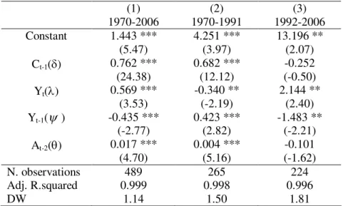
Table 1 reports the relevant results for specification (7) using GMM dynamic panel estimation. One can observe that the estimated coefficient for government debt is positive and statistically significant therefore not supporting the idea of Ricardian behaviour or that consumers are perceived as having infinite horizons. Still from Table 1 it is possible to see some evidence in favour of the existence of liquidity constrained consumers, eventually linked to less efficient capital markets, given the statistically significant estimated coefficient for the contemporaneous after tax income variable.
Since the institutional changes that occurred in the EU15 in the 1990s may have had an effect on how consumers perceive government indebtdness, alternative sub-sample periods are considered to take into account the signing of the European Union Treaty on 7 February 1992 in Maastricht, with the setting up of the convergence criteria. Therefore, I split the study period into the pre- and post-Maastricht, using 1992 as the first year of the new EU fiscal framework.9 Interestingly, although the rejection of the Ricardian hypothesis is maintained for the 1970-1991 period, it is no longer visible for the more recent 1992-2006 sub-period, when government debt no longer affects private consumption.
4.2 – The relevance of government indebtedness
Another possibility is to assess whether consumers choose to react differently according to the level of government debt reported by the government. This non-linear for the effect of debt on consumption can be rationalised as follows. In a high indebtedness environment, consumers anticipate the need for future higher taxes, in order for the government to finance debt repayments. Therefore, when taking their consumption decisions, consumers may bear in mind the importance of saving today to face more taxes tomorrow.
We can use the change in the debt-to-GDP ratio in order to assess the existence of a monotonic relation between government debt and private consumption. Therefore, specification (7) can be rewritten to include an interaction term between A and the change in the debt ratio, as follows:
1 1 2 2 2 2 1
it it it it it it it it
C
c
C
A
A
dratio
Y
Y
u
(8)where dratioit is the change in the debt-to-GDP ratio of country i in period t. In principle, one could expect a positive value for 1, capturing the positive wealth effect associated to government debt. On the other hand, the estimated value of 2 would be negative in order to capture the adverse effect of the size of government indebtedness.
We can also notice that the partial derivative of private consumption to government debt is given by
1 2 2
2 it
it it
C
dratio
A
(9)
which can provide us with a common estimate for the threshold of the change in the
debt-to-GDP ratio, that results in (9) being equal to zero:
________
1/ 2 0
dratio (provided that 1>0 and
2<0). For instance, when the change in the debt-to-GDP ratio is above the
________
dratio threshold a negative response from private consumption would then occur. On the other hand, as long as the change in the debt-to-GDP ratio stays below the critical threshold, private consumption would still have a positive response.
Table 2 reports in column 1 the estimation results for specification (8). We see that both estimated coefficients for the variables A and A*dratio are statistically significant and that
9
indeed we get the expected signs for each variable: 1>0 and 2<0. These results imply that after some threshold, measured by the change in government debt, consumers start seeing government indebtedness as more of a future problem for rather than attributing it any possible wealth characteristics. Computing such threshold from the solution that makes (10) equal to zero we get approximately 5.1 percentage points of GDP as the critical change in the debt-to-GDP ratio. From the full sample we can then observe that a negative link between private consumption and the change in government debt occurs for 60 cases out of the 489 panel observations.
[Table 2]
A slightly different specification is reported in column 2, Table 2, where the interaction term with government debt is now dratioupit, which is the change in the debt-to-GDP ratio of country i in period t when that change is a positive one. Again, we can observe rather similar estimation results with the critical threshold now being around 5.3 percentage points of GDP, which occurs in 56 cases of our sample. Finally, in column 3, an alternative specification interacts with the government debt the dummy variable dup, which assumes the value 1 when there is an increase in the debt-to-GDP ratio and 0 otherwise. The results for this alternative estimation also point to the possibility that consumers may become more Ricardian when facing increases in the debt ratios.
5 – Conclusion
This paper estimates private consumption Euler equations to test the debt neutrality hypothesis for the EU countries, using a panel data sample for the period 1970-2006. As for the empirical findings, one should note that debt carries a significant positive coefficient using the full country sample. Interestingly, although the rejection of the Ricardian hypothesis is maintained for the 1970-1991 sub-period, it is no longer visible for the more recent 1992-2006 sub-period, when government debt no longer affects private consumption.
Additionally, after some threshold, measured by the change in government debt, consumers start seeing government indebtedness as more of a future problem for them rather than attributing it any possible wealth characteristics. Indeed, increases of the debt-to-GDP ratio interacted with the debt variable negatively impnige on pirvate consumption. Therefore, if we ask the question, does higher government indebtedness imply a more Ricardian behaviour from European consumers, a cautious answer would be that there seems to be some evidence pointing that way. In other words, the idea of some consumer fiscal illusion seems to be lower the smaller the government indebtedness. A possible implication for economic policy, namely in the EU, would then be the notion that the Maastricht criteria on government debt may be looked upon with some latitude, in line with the existence of already “more indebted” countries in the Economic and Monetary Union.
Appendix
The aggregate consumption function, used in the paper,
1
0
1 (1 ) (1 )
1 i
t t t t t i
i
C Y A E Y
(A.1)can be lagged one period and multiplied by (1+)/(1-) to give
1 2 1 1
0
1 1 1 1
(1 ) (1 )
1 1 1 1
i
t t t t t i
i
C Y A E Y
.(A.2)Subtracting (A.2) from (A.1),
1 1
0
1 1
(1 ) (1 )
1 1
i
t t t t t t i
i
C C Y A E Y
2 1 1
0
1 1 1
(1 ) (1 )
1 1 1
i
t t t t i
i
Y A E Y
, (A.3)results in equation (2) of the text,
1 1 2 1
1 1 1
(1 ) (1 ) (1 )
1 1 1
t t t t t t t
C
C
A
A
Y
Y u
(A.4)
with
1
01 (1 )
1 i
t t t t i
i
u E E Y
. (A.5)Using the budget constraint lagged once,
t t t
t A Y C
A (1 ) 1 (A.6)
1 (1 ) 2 1 1
t t t t
A A Y C (A.7)
and substituting (A.7) in (A.4),
1 2 1 1 2
1 1
(1 ) (1 ) (1 )
1 1
t t t t t t
C C A Y C A
11
(1 ) 1
t t
Y Y
, (A.8)
2 2
1 1 2 2
1 (1 )
(1 ) (1 )
1 1
t t t t t
C C C A A
1 1 1(1 ) (1 )
1
t t t
Y Y Y
2 2
1 2
1 (1 )(1 ) (1 ) (1 ) (1 )
1 1 1 1
t t t
C C A
1(1 )(1 ) 1
(1 ) 1 1
t t
Y Y
, (A.10)
1 2
21 (1 )
1 (1 ) 1 1
1 1
t t t
C C A
11
(1 ) (1 ) 1
t t
Y Y
, (A.11)
1 2 2
11 (1 ) 1
1 (1 ) ( )
1 1 1
t t t t t t
C
C
A
Y
Y u
.(A.12)
which is equation (5) in the text.
Notice also that if ==0, then both (A.12) would colapse to
1
(1 )(1 )
t t t
C C u, (A.13)
with
1
0
1 1
i
t t t t i i
u E E Y
. (A.14)Annex: Data sources
Original series Ameco codes
Gross Domestic Product, at current market prices, national currency 1.0.0.0.UVGD
Gross Domestic Product, at 2000 market prices, national currency 1.1.0.0.OVGD
General government consolidated gross debt, Excessive deficit procedure (based on ESA 1995) and former definition (linked series), national currency
1.0.0.0.UDGGL 1.0.0.0.UDGGF Price deflator gross domestic product at market prices, (National currency:
2000 = 100)
3.1.0.0.PVGD
Private final consumption expenditure, at 2000 constant prices, national currency
1.1.0.0.OCPH
Current taxes on income and wealth (direct taxes); general government ESA 1995 - National currency- AMECO data class: Data at current prices
1.0.0.0.UTYG 1.0.0.0.UTYGF Taxes linked to imports and production (indirect taxes); general government
ESA 1995 - National currency- AMECO data class: Data at current prices
1.0.0.0.UTVG 1.0.0.0.UTVGF
Total population 1.0.0.0.NPTN
References
Akerlof, G. (2007). “The missing motivation in macroeconomics”, American Economic Review, 97 (1), 5-36.
Aschauer, D. (1985). “Fiscal Policy and Aggregate Demand,” The American Economic Review, 75 (1), March, 117-127.
Aschauer, D. (1988). “The Equilibrium Approach to Fiscal Policy,” Journal of Money, Credit and Banking, 20 (1), 41-62.
Barro, R. (1974). “Are Government Bonds Net Wealth?” Journal of Political Economy, 82 (6), 1095-117.
Barro, R. (1979). “On the Determination of Public Debt,” Journal of Political Economy, 87 (5), 940-971.
Becker, G. (1974). “A theory of social interactions,” Journal of Political Economy, 82 (6), 1063-1093.
Bernheim, D. (1987). “Ricardian Equivalence: An Evaluation of Theory and Evidence,” in Fischer, S. (ed.), NBER Macroeconomics Annual 1987, Cambridge, Mass., MIT Press, 263-315.
Blanchard, O. (1985). “Debt, deficits, and finite horizons,” Journal of Political Economy, 93, 223-247.
Brennan, H. and Buchanan, J. (1986). “The Logic of the Ricardian Equivalence Theorem,” in Buchanan, J; Rowley, C. and Tollison, R. (eds.), Deficits, Oxford, Basil Blackwell, 79-92.
Buiter, W. (1985). “A Guide to Public Sector and Deficits,” Economic Policy, 1, 13-79.
Buiter, W. and Tobin, J. (1979). “Debt Neutrality: A Brief Review of Doctrine and Evidence” in von Furstenberg, G. (ed.), Social Security versus Private Saving, Cambridge, Mass., Ballinger, 39-63.
Carmichael, (1982). “On Barro's theorem of debt neutrality: the irrelevance of net wealth,”
American Economic Review, 72 (1), 202-213.
Cushing, M. (1992). “Liquidity constraints and aggregate consumption behaviour,” Economic Inquiry, 30 (1), 134-53.
Dalamagas, B. (1992). “How Rival are the Ricardian Equivalence Proposition and the Fiscal Policy Potency View,” Scottish Journal of Political Economy, 39 (4), 457-476.
Diamond, P. (1965). “National Debt in a Neoclassical Growth Model,” The American Economic Review, 60, 1126-1150.
Evans, P. (1988). “Are Consumers Ricardian? Evidence for the United States,” Journal of Political Economy, 96 (5), 983-1004.
Evans, P. (1993). “Consumers are not Ricardian: evidence from nineteen countries,” Economic Inquiry, 31, 534-548.
Feldstein, M. (1982). “Government Deficits and Aggregate Demand,” Journal of Monetary Economics, 9 (1), 1-20.
Gupta, K. (1992). “Ricardian Equivalence and Crowding out in Asia,” Applied Economics, 24, 19-25.
Hall, R. (1978). “Stochastic Implications of the Life Cycle-Permanent Income Hypothesis: Theory and Evidence,” Journal of Political Economy, 86 (6), 971-987.
Haque, N. (1988). “Fiscal Policy and Private Sector Saving Behavior in Developing Countries”, IMF Staff Papers, 35 (2), 316-335.
Hayashi, F. (1982). “The Permanent Income Hypothesis: Estimation and Testing by Instrument Variables,” Journal of Political Economy, 90 (5), 895-916.
Himarios, D. (1995). “Euler Equation Tests of Ricardian Equivalence,” Economics Letters, 48, 165-171.
Hisao, C. (2002). Analysis of Panel Data, 2nd ed., Cambridge University Press.
Khalid, A. (1996). "Ricardian Equivalence: Empirical evidence from developing economies,"
Journal of Development Economics, 51 (2), 413-432.
Leiderman, L. and Razin, A. (1988). “Testing Ricardian Neutrality with an Intertemporal Stochastic Model,” Journal of Money, Credit and Banking, 20 (1), 1-21.
Lopez, J.; Schmidt-Hebbel, K. and Servén, L. (2000). "How effective is fiscal policy in raising national saving?" Review of Economics and Statistics, 82 (2), 226-238.
O’Driscoll, G. P. (1977). “The Ricardian Nonequivalence Theorem,” Journal of Political Economy, 85 (1), 207-210.
Phelps, E. (1982). “Cracks on the Demand Side: A Year of Crisis in theoretical Macroeconomics,” American Economic Review, 72 (2), 378-381.
Ricardo, D. (1817). On the Principles of Political Economy and Taxation, in P. Sraffa (ed.),
The works and correspondence of David Ricardo, Volume I, 1951, Cambridge University Press, Cambridge.
Samuelson, P. (1958). “An Exact Consumption-Loan Model of Interest with or without the Social Contrivance of Money,” Journal of Political Economy, 66 (6), 467-482.
Seater, J. (1993). “Ricardian Equivalence,” Journal of Economic Literature, 31, March, 142-190.
Table 1 – Private consumption Euler equation estimation (1) 1970-2006 (2) 1970-1991 (3) 1992-2006
Constant 1.443 ***
(5.47)
4.251 *** (3.97)
13.196 ** (2.07)
Ct-1() 0.762 ***
(24.38)
0.682 *** (12.12)
-0.252 (-0.50)
Yt() 0.569 ***
(3.53)
-0.340 ** (-2.19)
2.144 ** (2.40)
Yt-1( ) -0.435 ***
(-2.77)
0.423 *** (2.82)
-1.483 ** (-2.21)
At-2() 0.017 ***
(4.70)
0.004 *** (5.16)
-0.101 (-1.62)
N. observations 489 265 224
Adj. R.squared 0.999 0.998 0.996
DW 1.14 1.50 1.81
Notes: GMM, dynamic panel estimation, t statistics are in brackets. *, **, *** - Significant at the 10, 5 and 1 per cent level respectively.
Table 2 – Private consumption Euler equation estimation, the relevance of government indebtedness (1970-2006)
(1) (2) (3)
Constant 4.750 ***
(3.13)
4.258 *** (3.67)
4.357 *** (4.24)
Ct-1() 0.394 **
(2.31)
0.490 *** (4.13)
0.500 *** (5.01)
Yt () 1.817 ***
(2.78)
1.591 *** (3.15)
1.188 *** (3.35)
Yt-1( ) -1.524 ***
(-2.56)
-1.355 *** (-2.87)
-0.956 *** (-2.88) At-2() 0.022 **
(2.35)
0.034 *** (3.43)
0.042 *** (4.09) At-2*dratio() -0.004 **
(-2.41)
At-2*dratioup() -0.007 ***
(-2.78)
At-2*dup() -0.049 ***
(-3.22)
5.1 5.3 -
N. observations 489 489 489
Adj. R.squared 0.996 0.997 0.998
DW 1.32 1.33 1.41