UNIVERSIDADE DA BEIRA INTERIOR
Engenharia
Development of an Open Source Software Tool for
Propeller Design in the MAAT Project
Desenvolvimento de uma Ferramenta Computacional de
Código Aberto para Projeto de Hélices no Âmbito do
Projeto MAAT
João Paulo Salgueiro Morgado
Tese para obtenção do Grau de Doutor em
Engenharia Aeronáutica
(3º ciclo de estudos)
Orientador: Prof. Doutor Miguel Ângelo Rodrigues Silvestre Coorientador: Prof. Doutor José Carlos Páscoa Marques
A execução deste trabalho só foi possível devido à colaboração, disponibilidade e empenho de algumas pessoas às quais quero desde já manifestar o meu mais sincero agradecimento. Ao Professor Miguel Silvestre, pela orientação neste trabalho, pelos conhecimentos que me transmitiu, pelo rigor científico com que sempre desenvolveu o trabalho e por me ter incutido um espírito crítico. Agradeço-lhe também pela sua amizade, por toda a disponibilidade e atenção que sempre dispensou ao longo destes anos.
Ao Professor José Páscoa, pela sua co-orientação neste trabalho, pela sua constante disponibilidade, pelos conhecimentos que me transmitiu e pelos conselhos que me deu. Quero ainda agradecer-lhe o espaço que me disponibilizou no ClusterDEM, permitindo que este trabalho fosse desenvolvido num ambiente calmo e confortável.
Ao Sr. Rui, ao Pedro Santos e ao Pedro Alves pelo apoio prestado na parte experimental deste trabalho e pelo seu empenho na resolução dos problemas que foram surgindo.
Ao Carlos, à Galina, ao Shyam, ao Jakson e ao Frederico, com quem partilhei o espaço de trabalho do ClusterDEM, pela disponibilidade sempre demonstrada e ainda pela possibilidade de ter partilhado estes anos com pessoas de diferentes culturas e costumes.
Ao Amilcar, ao Rui, ao Mahdi e ao Luís por tudo o que partilhámos ao longo destes anos, pelo apoio que sempre me deram nos momentos menos bons, pelas discussões mais ou menos científicas que tivemos e sobretudo pela vossa amizade.
A ti, Andreia, por tudo. Por me fazeres sorrir, por estares sempre a meu lado por me aturares e por me ajudares a ver sempre o lado mais positivo das coisas. O meu obrigado não é suficiente por todo o carinho que demonstras por mim.
À minha Mãe, ao meu Pai e às minhas Irmãs pois sem vocês nada disto teria sido possivel. Obrigado por estarem sempre presentes, pela compreensão, pelo constante apoio e pelo encorajamento ao longo destes anos. Não é possível agradecer tudo o que fazem por mim.
A todos o meu Muito Obrigado!
Support
The present work was performed as part of Project MAAT (Ref. No. 285602) supported by
European Union Seventh Framework Programme. Part of the work was also supported by C-MAST – Center for Mechanical and Aerospace Sciences and Technologies, Portuguese
Nesta tese é apresentado o desenvolvimento de um novo código para projeto e análise de hélices, capaz de prever adequadamente o desempenho a baixos números de Reynolds. O JBLADE foi desenvolvido partindo dos códigos QBLADE e XFLR5 e utiliza uma versão aperfeiçoada da teria do elemento da pá que contém um novo modelo que considera o equilíbrio tridimensional do escoamento. O código permite que a pá seja introduza como um número arbitrário de secções, caracterizadas pela sua posição radial, corda, ângulo de incidência, comprimento, perfil e ainda pela polar 360º associada ao perfil. O código permite uma visualização gráfica em 3D da pá, ajudando o utilizador a detetar possíveis inconsistências. O JBLADE também permite uma visualização direta dos resultados das simulações através de um interface gráfico, tornado o código acessível e de fácil compreensão. Além disso, a interligação entre os diferentes módulos do JBLADE evita operações demoradas de importação e exportação de dados, diminuindo assim possíveis erros criados pelo utilizador. O código foi desenvolvido como um código aberto, para a simulação de hélices, e que tem a capacidade de estimar o desempenho de uma determinada geometria de hélice nas condições de operação do seu ponto de projeto e fora do seu ponto de projeto. O trabalho de desenvolvimento aqui apresentado foi focado no projeto de hélices para dirigíveis de grande altitude no âmbito do projeto MAAT (Multibody Advanced Airship for Transportation). O software foi validado para diferentes tipos de hélice, provando que pode ser utilizado para projetar e otimizar hélices para diferentes finalidades.
São apresentadas a derivação e validação do novo modelo de equilíbrio tridimensional do escoamento. Este modelo de equilíbrio 3D tem em conta o possível movimento radial do escoamento ao longo do disco da hélice, melhorando as estimativas de desempenho do software. O desenvolvimento de um novo método para a estimativa do coeficiente de arrasto dos perfis a 90º, permitindo uma melhor modelação do desempenho pós-perda é também apresentado. Diferentes modelos de pós perda presentes na literatura e originalmente desenvolvidos para a indústria das turbinas eólicas foram implementados no JBLADE e a sua aplicação a hélices para melhorar a estimativa do desempenho foi analisada. Os resultados preliminares mostraram que a estimativa de desempenho das hélices pode ser melhorada, utilizando estes modelos de pós-perda. Uma metodologia de projeto inverso, baseada no mínimo das perdas induzidas foi implementado no JBLADE, de modo a ser possível obter hélices com geometrias otimizadas para um dado ponto de projeto. Além disto, um módulo de cálculo estrutural foi também implementado, permitindo estimar o peso das pás, a deformação das mesmas, quer em termos de flexão, quer em termos de torção, devido à tração gerada pela própria hélice e aos momentos do perfil. Para validar as estimativas de desempenho do JBLADE foram utilizadas hélices originalmente apresentadas nos relatórios técnicos NACA, nomeadamente no relatório técnico 594 e 530. Estas hélices foram simuladas no JBLADE e os resultados foram comparados com os dados experimentais e com as estimativas de desempenho
foram também validados, através da comparação com outros resultados numéricos.
De modo a verificar a fiabilidade do código XFOIL usado no JBLADE para previsão das características dos perfis das pás, o modelo de turbulência k-ω Shear Stress Transport e uma versão reformulada do modelo de transição k-kl-ω foram utilizados em simulações RANS para comparação dos resultados do desempenho aerodinâmico de perfis. Os resultados mostraram que o código XFOIL dá uma estimativa de desempenho mais próxima dos dados obtidos experimentalmente do que os modelos RANS CFD, provando que pode ser utilizado no JBLADE como ferramenta de estimava de desempenho aerodinâmico dos perfis.
Em vez da tradicional prescrição do coeficiente de sustentação ao longo da pá para melhor L/D, foi utilizado os pontos de melhor L3/2/D para o projeto de uma hélice para o dirigível cruzador
do projeto MAAT. Os procedimentos de otimização empregados ao longo do processo de projeto destas hélices para utilização em grandes altitudes são também descritos. As hélices projetadas com o JBLADE foram analisadas e os resultados obtidos foram comparados com simulações convencionais de dinâmica de fluidos computacional, uma vez que não existem dados experimentais para estas geometrias em particular. Foram utilizadas duas aproximações diferentes de modo a obter duas geometrias finais. Foi mostrado que esta nova abordagem de projeto de hélices leva à minimização da corda necessária ao longo da pá, enquanto a tração e a eficiência da hélice são maximizadas.
Foi desenvolvida uma nova instalação experimental para ensaio e caracterização de hélices de baixo número de Reynolds no âmbito do projeto MAAT, que foi posteriormente utilizada para desenvolver e validar ferramentas numéricas para projeto destas hélices. Além da descrição do desenvolvimento da instalação experimental, é também apresentada a validação da mesma, através da comparação das medições de diferentes hélices com dados experimentais presentes na literatura, obtidos em diferentes instalações de referência. Foi construída e testada uma réplica da hélice APC 10”x7” SF, fornecendo dados adicionais para a validação do JBLADE. É ainda apresentado o processo de desenho da réplica no software CAD e de construção dos moldes e do protótipo da hélice. Os resultados mostraram uma boa concordância entre as estimativas do JBLADE e as medições experimentais. Assim, conclui-se que o JBLADE pode ser utilizado para projetar e estimar o desempenho das hélices que poderão ser utilizadas pelo dirigível cruzador do MAAT bem como em outras aplicações.
Palavras-chave
JBLADE Software, Teoria do Elemento de Pá, Correções Pós-Perda, Equilíbrio 3D do escoamento, Projeto Inverso de Hélices, Simulação de Hélices em Dinâmica de Fluidos
This thesis presents the development of a new propeller design and analysis software capable of adequately predicting the low Reynolds number performance. JBLADE software was developed from QBLADE and XFLR5 and it uses an improved version of Blade Element Momentum (BEM) theory that embeds a new model for the three-dimensional flow equilibrium. The software allows the introduction of the blade geometry as an arbitrary number of sections characterized by their radial position, chord, twist, length, airfoil and associated complete 360º angle of attack range airfoil polar. The code provides a 3D graphical view of the blade, helping the user to detect inconsistencies. JBLADE also allows a direct visualization of simulation results through a graphical user interface making the software accessible and easy to understand. In addition, the coupling between different JBLADE modules avoids time consuming operations of importing/exporting data, decreasing possible mistakes created by the user. The software is developed as an open-source tool for the simulation of propellers and it has the capability of estimating the performance of a given propeller geometry in design and off-design operating conditions. The current development work was focused in the design of airship propellers. The software was validated against different propeller types proving that it can be used to design and optimize propellers for distinct applications.
The derivation and validation of the new 3D flow equilibrium formulation are presented. This 3D flow equilibrium model accounts for the possible radial movement of the flow across the propeller disk, improving the performance prediction of the software. The development of a new method for the prediction of the airfoil drag coefficient at a 90 degrees angle of attack for a better post-stall modelling is also presented. Different post-stall methods available in the literature, originally developed for wind turbine industry, were extended for propeller analysis and implemented in JBLADE. The preliminary analysis of the results shows that the propeller performance prediction can be improved using these implemented post-stall methods. An inverse design methodology, based on minimum induced losses was implemented in JBLADE software in order to obtain optimized geometries for a given operating point. In addition a structural sub-module was also integrated in the software allowing the estimation of blade weight as well as tip displacement and twist angle changes due to the thrust generation and airfoil pitching moments. To validate the performance estimation of JBLADE software, the propellers from NACA Technical Report 530 and NACA Technical Report 594 were simulated and the results were checked against the experimental data and against those of other available codes. The inverse design and structural sub-module were also validated against other numerical results.
To verify the reliability of XFOIL, the XFOIL Code, the Shear Stress Transport k-ω turbulence model and a refurbished version of k-kl-ω transition model were used to estimate the airfoil aerodynamic performance. It has been shown that the XFOIL code gives the closest prediction
Software as airfoil’s performance estimation tool.
Two different propellers to use on the MAAT high altitude cruiser airship were designed and analysed. In addition, the design procedure and the optimization steps of the new propellers to use at such high altitudes are also presented. The propellers designed with JBLADE are then analysed and the results are compared with conventional CFD results since there is no experimental data for these particular geometries. Two different approaches were used to obtain the final geometries of the propellers, since, instead of using the traditional lift coefficient prescription along the blade, the airfoil’s best L3/2/D and best L/D were used to
produce different geometries. It was shown that this new first design approach allows the minimization of the chord along the blade, while the thrust and propulsive efficiency are maximized.
A new test rig was developed and used to adequately develop and validate numerical design tools for the low Reynolds numbers propellers. The development of an experimental setup for wind tunnel propeller testing is described and the measurements with the new test rig were validated against reference data. Additionally, performance data for propellers that are not characterized in the existing literature were obtained. An APC 10”x7” SF replica propeller was built and tested, providing complementary data for JBLADE validation. The CAD design process as well as moulds and propeller manufacture are also described. The results show good agreement between JBLADE and experimental performance measurements. Thus it was concluded that JBLADE can be used to design and calculate the performance of the MAAT project high altitude cruiser airship propellers.
Keywords
JBLADE Software, Blade Element Momentum Theory, Post-Stall Corrections, 3D Flow Equilibrium, Propeller Inverse Design, CFD Propeller Simulation, Wind Tunnel Testing
Este trabalho apresenta o desenvolvimento de um nova ferramenta para projeto e análise do desempenho de hélices operando a baixos números de Reynolds. A ferramente desenvolvida é um software que contém uma interface gráfica e que foi desenvolvido tendo como base os softwares QBLADE e XFLR5, já existentes. A inovação deste código consiste na implementação de uma versão melhorada da teoria do elemento de pá, normalmente utilizada por outros códigos de projeto e análise de desempenho de hélices, que tem em conta um equilíbrio tri-dimensional do escoamento, contabilizando assim a rotação da esteira, e melhorando as previsões de desempenho das hélices.
Este trabalho foi desenvolvido no âmbito do projeto europeu Multibody Advanced Airship for Transport (MAAT), que envolveu mais de 15 entidades, e que pretende implementar um novo modelo de transporte através da utilização de dirigíveis. Neste modelo são utilizados 2 tipos de dirigíveis: um crusador, que operará entre os 15 000- 16 000 m de altitude e um outro tipo de dirigivel que será responsável por fazer a ligação entre o solo e o crusador. Ora, como apresentado ao longo do documento, as hélices têm vindo a ser utilizadas em veículos com uma altitude de operação semelhante, pelo que é essencial o desenvolvimento de uma ferramenta fiável para projectar e analisar as hélices do crusador do projeto MAAT.
Durante o estudo e análise do estado atual das teorias aplicavéis a hélices, chegou-se à conclusão que era possível melhorar essas teorias. Este modelo de equilíbrio tri-dimensional tem em conta o possível movimento radial do escoamento ao longo do disco da hélice, melhorando as estimativas de desempenho do software Além disto, como as hélices têm ângulos de torção bastante elevados, principalmente na zona da raíz, os perfis das pás estão muitas vezes a operar em regime pós-perda, e os códigos númericos utilizados para prever o seu desempenho nem sempre fornecem dados fidedignos acerca do desempenho dos mesmos. O JBLADE utiliza um método que consiste na extrapolação dos valores do coeficiente de sustentação e do coeficiente de arrasto apresentado na literatura. Neste modelo, a previsão do valor do coeficiente de arrasto tem uma importância vital para uma correcta extrapolação deste mesmo coefficiente, podendo levar a diferenças significativas na previsão de desempenho da hélice. Assim, de modo a melhorar a previsão de desempenho da hélice foi desenvolvido um novo método para estimar o coeficiente de arrasto de um perfil a um angulo de ataque de 90º. Este método baseia-se no raio do bordo de ataque do perfil e foi também incorporado no JBLADE. Foram também implementados no JBLADE diferentes modelos de pós perda, originalmente desenvolvidos para a indústria de turbinas eólicas que como demonstrados, melhoram a previsão de desempenho para baixas razões de avanço. Foram comparados diferentes modelos e os resultados foram analisados e discutidos. Estes modelos estão disponíveis no JBLADE, podendo ser utilizados ou não na simulação da hélice, conforme as preferências do utilizador.
projeto inverso descrito na literatura. Foram feitas algumas modificações ao método original, nomeadamente através da utilização do ponto de melhor L/D e L3/2/D dos perfis, permitindo
que a corda necessária para produzir uma determinada tração seja menor. Este processo foi validado através da comparação dos dados obtidos no JBLADE com outros dados disponíveis na literatura bem como com outros códigos disponíveis. Esta implementação do método de projeto inverso foi depois utilizado para projetar uma hélice para aplicação no dirigível crusador do projeto MAAT.
Uma vez que as hélices que serão utilizadas no dirigível do projeto MAAT serão bastante grandes, é importante assegurar que não sofrerão uma deformação excessiva, que poderá levar à sua destruição. Assim, foi implementado um módulo de cálculo estrutural, no qual a pá da hélice é considerada uma viga encastrada. Esta viga está sujeita a um momento flector e a um momento torsor, que surgem devido à geração de tração pela própria pá. Depois de uma análise aerodinâmica da pá, o utilizador pode definir um material para a mesma, bem como selecionar um conceito de construção entre os disponíveis e escolher o ponto para o qual quer analizar a deformação a que a pá está sujeita. Os resultados são apresentados na forma de gráficos de deslocamento e incremento ao ângulo de torção ao longo da envergadura da pá. Este módulo estrutural permite que o utilizador leve a cabo uma iteração adicional durante o projecto, e que garante que a pá não deformará excessivamente quando estiver em operação. O módulo estrutural permite ainda estimar o peso e o volume de cada pá, algo importante para o caso concreto do dirigível MAAT, uma vez que terá um grande número de hélices.
O JBLADE é um software, desenvolvido como um código open source, escrito em linguagem C++/QML e compilado utilizando Qt® Creator. O software mantém todas as funcionalidades originais do módulo XFOIL originalmente desenvolvidas no XFLR5, que permitem o projecto e a optimização de perfis para um dado ponto de projecto. O JBLADE possui uma interface gráfica e através da qual é possível executar todos os passos necessários ao projeto e análise de desempenho de uma hélice. O software permite que a pá seja introduza como um número arbitrário de secções, caracterizadas pela sua posição radial, corda, ângulo de incidência, comprimento, perfil e ainda pela polar 360º associada ao perfil. Este software permite também uma visualização e manipulação gráfica em 3 dimensões da pá/hélice, ajudando o utilizador a detetar possíveis inconsistências. O JBLADE também permite uma visualização direta e gráfica dos resultados das simulações de desempenho da hélice, tornado o código acessível e intuitivo. Uma vez que todos os módulos internos do JBLADE estão interligados, são evitadas operações demoradas de importação e exportação de dados, diminuindo assim possíveis erros criados pelo utilizador durante este processo. O código foi desenvolvido como um código aberto, para a simulação de hélices, e que tem a capacidade de estimar o desempenho de uma determinada geometria nas condições de operação do seu ponto de projeto e fora desse ponto de projeto.
foram utilizadas diferentes geometrias, provando que o JBLADE pode ser utilizado para projetar e otimizar hélices para diferentes finalidades.
O procedimento de simulação de uma hélice foi validado, garantindo que pode ser utilizado um ponto intermédio e a distribuição correspondente dos números de Reynolds e de Mach. Foi ainda validado o número de pontos necessário para definir um perfil no sub-módulo XFOIL, mostrando que acima de 200 pontos não existem diferenças significativas no cálculo do desempenho do perfil, para um dado número de Reynolds. O novo método anteriormente apresentado para estimativa da previsão do coeficiente de arrasto foi também validado, e o seu efeito na previsão do desempenho das hélices foi demonstrado. O JBLADE foi ainda extensivamente validado através da comparação com dados experimentais apresentados na literatura, nomeadamente e com outros códigos numéricos disponíveis.
Para garantir que o XFOIL poderia ser utilizado como ferramenta de previsão do desempenho de um perfil para um dado ponto de operação, foram feitas simulações para os perfis E387 e S1223 e comparadas com dados obtidos através de simulações de dinâmica dos fluidos computacional. Nestas simulações foram utilizados o modelo de turbulência k-ω Shear Stress Transport (SST) e uma versão remodelada do modelo de transição k-kl-ω. O modelo de transição k-kl-ω foi utilizado uma vez que prever o ponto de transição ao longo da corda é essencial para conseguir calcular correctamente o desempenho dos perfis que operam a baixos números de Reynolds (60 000<Re<500 000). Os resultados mostraram que o XFOIL consegue prever o desempenho dos perfis tão bem quanto os modelos de turbulência e de transição utilizados nas simulações de dinâmica dos fluidos computacional. Além disso, o XFOIL tem ainda a vantagem de as simulações serem mais rápidas e de necessitar de muito menos recursos computacionais quando comparado com as simulações de dinâmica dos fluidos computacional. O XFOIL pode, assim, continuar a ser utilizado como ferramenta de cálculo para o desempenho dos perfis que serão utilizados ao longo das pás da hélice.
Durante este trabalho foi ainda desenvolvida uma nova instalação experimental, que foi posteriormente utilizada na validação do JBLADE. Esta instalação experimental, aplicada no túnel de vento do Departamento de Ciências Aeroespaciais da Universidade da Beira Interior foi validada através da comparação das medições obtidas para uma hélice com dados experimentais obtidos para essa mesma hélice noutras instalações experimentais. Além da validação da instalação experimental, foi construída e testada uma réplica da hélice APC 10”x7” SF, fornecendo dados adicionais para a validação do JBLADE. É apresentado todo o processo de desenho da réplica da hélice APC 10”x7” SF no software CAD bem como os passos necessários para a construção dos moldes. Foram desenhados 2 moldes fémea no software CATIA e posteriormente maquinados utilizando uma fresadora controlada por computador. Para obter a hélice final foi colocada fibra de carbono no interior dos moldes, sendo estes posteriormente fechados. Foi então introduzida resina epoxy, de modo a preencher todas as
experimentais foram depois comparaddos com as simulações efectuadas no JBLADE, mostrarando uma boa concordância entre as estimativas do JBLADE e as medições experimentais. Através de tudo o que foi anteriormente apresentado foi possivel concluir que que o JBLADE pode ser utilizado para projetar e estimar o desempenho de hélices, que entre outras aplicações, poderão ser utilizadas pelo dirigível cruzador do projecto MAAT.
Agradecimentos ... vii Support ... vii Resumo ... ix Palavras-chave ... x Abstract... xi Keywords ... xii
Resumo Alargado ... xiii
Table of Contents ... xvii
List of Figures ... xxi
List of Tables ... xxvii
Nomenclature ... xxix
Latin Terms ... xxix
Greek Symbols ... xxxii
Acronyms ... xxxiii Chapter 1 ... 1 1.1 -Motivation ... 1 1.2 - Objectives ... 2 1.3 -Contributions ... 2 1.4 - Thesis Outline ... 3 Chapter 2 ... 5
2.1 - Historical Developments of Propeller Theory ... 5
2.2 -Present Status of Propeller Aerodynamics ... 7
2.3 - Available Propeller Design Codes ... 8
2.4 -Propeller Theory ... 8
2.4.1 - Momentum Theory ... 8
2.4.2 - Blade Element Theory ... 10
2.4.3 - Blade Element Momentum Theory ... 12
Prandtl Tip and Hub Losses Corrections ... 13
Post Stall Models ... 14
2.4.4 - Propeller Momentum Theory with Slipstream Rotation ... 17
2.4.5 - Propeller Inverse Design Methodology ... 18
2.5 -Forces acting on a Propeller ... 20
2.5.1 - Volume and Blade Mass Estimation ... 22
2.5.2 - Blade Bending Estimation ... 23
2.5.3 - Blade Twist Deformation ... 24
2.6 -Present Research Contributions to Propeller Aerodynamics Modelling ... 25
2.6.1 - New 3D Flow Equilibrium Model ... 25
Chapter 3 ... 31
3.1 - Software Overview... 31
3.1.1 - Airfoil design and analysis ... 32
3.1.2 - 360º AoA Polar extrapolation ... 33
3.1.3 - Blade definition ... 34
Propeller inverse design ... 35
3.1.4 - Parametric simulation ... 36
3.1.5 - Propeller definition and simulation ... 37
Number of blade elements... 39
Foil interpolation ... 39
Fluid density and viscosity ... 40
Convergence criteria ... 40
Relaxation factor ... 40
Reynolds Number Correction ... 40
3.1.6 - Structural sub-module ... 41
Creating and editing materials ... 41
3.2 -JBLADE Software Validation ... 42
3.2.1 - Propeller Geometries... 42
NACA Technical Report 594 ... 42
NACA Technical Report 530 ... 42
Adkins and Liebeck Propeller ... 43
APC 11”x4.7” ... 43
3.2.2 - Simulation Procedure Validation ... 44
3.2.3 - Methods for Drag Coefficient at 90º Prediction Validation ... 49
NACA Technical Report 594 ... 49
NACA Technical Report 530 ... 51
3.2.4 - Post-Stall Models ... 54
NACA Technical Report 594 ... 54
3.2.5 - Inverse Design Methodology Validation ... 57
Adkins and Liebeck Propeller ... 57
3.2.6 - JBLADE vs Other BEM Codes ... 58
NACA Technical Report 594 ... 58
NACA Technical Report 530 ... 62
Adkins and Liebeck Propeller ... 66
APC 11”x4.7” Propeller ... 68
3.2.7 - Structural Sub-Module Validation ... 70
CATIA simulation validation ... 71
4.1 -Theoretical Formulation ... 84
4.1.1 - k-kl-ω model ... 84
4.1.2 - Shear Stress Transport k-ω model ... 87
Low Reynolds Correction ... 88
4.1.3 - XFOIL ... 88 4.2 - Numerical Procedure ... 89 4.2.1 - Mesh Generation ... 89 4.2.2 - Boundary Conditions ... 89 4.3 -Results ... 90 4.3.1 - E387 Airfoil ... 90 4.3.2 - S1223 Airfoil ... 93 Chapter 5 ... 95
5.1 -High Altitude Propellers ... 95
5.1.1 - Egrett ... 95 5.1.2 - Condor ... 96 5.1.3 - Pathfinder ... 96 5.1.4 - Perseus ... 96 5.1.5 - Strato 2C ... 96 5.1.6 - Theseus ... 97
5.2 - MAAT Cruiser Requirements ... 97
5.3 -Propeller Design and Optimization ... 98
5.3.1 - Airfoil Development ... 99
5.4 -A New High Altitude Propeller Geometry Design Concept ... 100
Chapter 6 ... 103
6.1 -APC 10”x7” SF Propeller ... 103
6.1.1 - CFD procedure ... 104
6.1.2 - 3D Flow equilibrium validation ... 107
6.1.3 - Performance prediction ... 107
6.2 -MAAT Cruiser Propeller ... 109
6.2.1 - CFD procedure ... 109
6.2.2 - Performance prediction ... 113
Chapter 7 ... 117
7.1 -Experimental Setup ... 117
7.1.1 - Wind tunnel ... 117
7.1.2 - Thrust Balance Concept ... 118
7.1.3 - Thrust and Torque Measurements ... 119
7.1.4 - Propeller rotation speed measurement ... 120
7.1.5 - Free stream flow speed measurement ... 120
7.1.6 - Balance Calibration ... 121
7.2.1 - Boundary corrections for propellers ... 124
7.2.2 - Motor fixture drag correction ... 125
7.3 -Validation of the Test Rig ... 126
7.3.1 - Sampling time independence ... 126
7.3.2 - Measurements repeatability ... 127
7.3.3 - Propeller performance data comparison... 129
APC 10”x4.7” Slow Flyer ... 129
APC 11”x5.5” Thin Electric ... 131
7.3.4 - Uncertainty Analysis ... 136
7.4 - APC 10”x7” SF Propeller Inverse Design ... 138
7.4.1 - Propeller CAD inverse design ... 138
7.4.2 - Moulds manufacture ... 139
7.4.3 - Propeller manufacture ... 140
7.5 - Results and Discussion ... 141
Chapter 8 ... 145
8.1 - Summary and conclusions ... 145
8.2 -Future Works ... 147
Bibliography ... 149
Appendix A ... 157
A.1 – Freestream Velocity ... 159
A.2 – Advance Ratio ... 159
A.3 – Thrust Coefficient ... 159
A.4 – Power Coefficient ... 160
A.5 – Propeller Efficiency ... 160
Appendix B ... 161
List of Publications ... 163
Peer Reviewed Journal Papers ... 163
Peer Reviewed International Conferences ... 164
Peer Reviewed National Conferences ... 164
B.I – Validation of New Formulations for Propeller Analysis ... 165
B.II – Propeller Performance Measurements at Low Reynolds Numbers ... 177
B.III – A Comparison of Post-Stall Models Extended for Propeller Performance Prediction 191 B.IV – High altitude propeller design and analysis ... 205
Figure 2.1 - Propeller Stream-tube (Rwigema, 2010). ... 9
Figure 2.2 – Geometry of rotor annulus (Prouty, 2003). ... 10
Figure 2.3 - Blade element geometry and velocities at an arbitrary radius position (Drela, 2006) ... 11
Figure 2.4 - Flowchart of inverse design procedure in JBLADE. ... 21
Figure 2.5 – (a) Illustration of propeller torque bending force and propeller centrifugal force. Reproduced from Mechanics Powerplant Handbook (1976) (b) Illustration of propeller trust bending force. ... 22
Figure 2.6 – Scheme of a cantilevered beam with a group of arbitrary positioned loads. ... 23
Figure 2.7 – Illustration of a beam subjected to a twisting moment. ... 24
Figure 2.8 - Measured airfoil drag coefficient at 90 degrees AoA vs airfoil leading edge radius. The airfoil data correspond to those of Table 2.2. ... 28
Figure 2.9 - Comparison between original correlation, described by Timmer (2010) and improved correlation. The airfoil data correspond to those of Table 2.2. ... 29
Figure 3.1 - JBLADE software structure representing the internal sub-modules interaction. . 32
Figure 3.2 - XFOIL sub-module in JBLADE. ... 33
Figure 3.3 - 360 Polar Extrapolation Sub-Module Screen ... 34
Figure 3.4 - Blade Definition Sub-Module ... 35
Figure 3.5 - Blade definition/inverse design sub-module in JBLADE. ... 36
Figure 3.6 – Parametric Simulation Sub-Module in JBLADE. ... 36
Figure 3.7 – Simulation sub-module overview. ... 37
Figure 3.8 - Flowchart of simulation procedure in JBLADE. ... 38
Figure 3.9 - Simulation definition dialog box. ... 38
Figure 3.10 – Representation of the sections and the sinusoidal spaced elements along the blade. ... 39
Figure 3.11 – Structural sub-module overview. ... 41
Figure 3.12 – New material definition dialog box. ... 41
Figure 3.13 - NACA Technical Report No. 594 (Theodorsen et al., 1937) propeller (a) propeller geometry (b) propeller visualization in JBLADE. ... 42
Figure 3.14 - NACA Technical Report No. 530 (Gray, 1941) 6267A-18 propeller (a) propeller geometry (b) propeller visualization in JBLADE. ... 43
Figure 3.15 - Propeller geometry presented by Adkins & Liebeck (1994) (a) propeller geometry (b) propeller visualization in JBLADE ... 43
Figure 3.16 - APC 11”x4.7” propeller(Brandt et al., 2014) (a) propeller geometry (b) Illustration of the propeller inside JBLADE ... 44
Figure 3.17 – E387 airfoil polars. (a) Validation of polar calculation using different number of points to define the airfoil in XFOIL (b) Comparison between XFOIL and experimental studies (Selig & Guglielmo, 1997) different Reynolds numbers ... 45
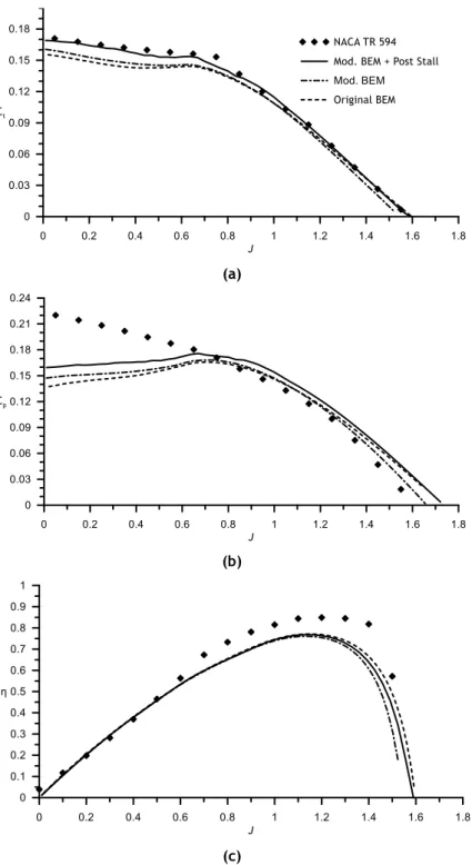
Figure 3.19 - Validation of calculations for the Propeller “C” of NACA TR 594 (Theodorsen et al., 1937) using a distribution of averaged Reynolds and Mach Numbers along the blade: (a) thrust coefficient (b) power coefficient, (c) propeller efficiency. ... 47 Figure 3.20 - Modelation influence on the simulated propeller performance: (a) thrust coefficient (b) power coefficient (c) propeller efficiency. ... 48 Figure 3.21 – Influence of the 360 polars extrapolation in the propeller performance and comparison with data from NACA TR 594 for θ75=45°: (a) thrust coefficient (b) power coefficient
(c) propeller efficiency. ... 50 Figure 3.22 - Influence of the 360 polars extrapolation in the propeller performance and comparison with data from NACA TR 530 for θ75=30°: (a) thrust coefficient (b) power coefficient
(c) propeller efficiency. ... 51 Figure 3.23 - Influence of the 360 polars extrapolation in the propeller performance and comparison with data from NACA TR 530 for θ75=40° (a) thrust coefficient (b) power coefficient,
(c) propeller efficiency. ... 52 Figure 3.24 - Influence of the 360 polars extrapolation in the propeller performance and comparison with data from NACA TR 530 for θ75=50° (a) thrust coefficient (b) power coefficient,
(c) propeller efficiency. ... 53 Figure 3.25 - Comparison between data predicted by JBLADE using different post-stall models and data from NACA TR No. 594 (Theodorsen et al., 1937) for θ75=30° (a) thrust coefficient (b)
power coefficient (c) propeller efficiency. ... 55 Figure 3.26 - Comparison between data predicted by JBLADE using different post-stall models and data from NACA TR No. 594 (Theodorsen et al., 1937) for θ75=45° (a) thrust coefficient (b)
power coefficient (c) propeller efficiency. ... 56 Figure 3.27 - Validation of the inverse design methodology. (a) blade incidence angle (b) chord ... 57 Figure 3.28 - Results of NACA TR 594 (Theodorsen et al., 1937) for θ75=15° (a) thrust coefficient
(b) power coefficient (c) propeller efficiency. ... 59 Figure 3.29 - Results of NACA TR 594 (Theodorsen et al., 1937) for θ75=30° (a) thrust coefficient
(b) power coefficient (c) propeller efficiency. ... 60 Figure 3.30 – Results of NACA TR 594 (Theodorsen et al., 1937) for θ75=45° (a) thrust coefficient
(b) power coefficient (c) propeller efficiency. ... 61 Figure 3.31 – Results of NACA TR 530 (Gray, 1941) for θ75=30° (a) thrust coefficient (b) power
coefficient (c) propeller efficiency. ... 63 Figure 3.32 - Results of NACA TR 530 (Gray, 1941) for θ75=40° (a) thrust coefficient (b) power
coefficient (c) propeller efficiency. ... 64 Figure 3.33 - Results of NACA TR 530 (Gray, 1941) for θ75=50° (a) thrust coefficient (b) power
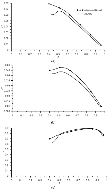
coefficient (c) propeller efficiency. ... 65 Figure 3.34 - Comparison between data predicted by JBLADE and data obtained from Adkins &
for an APC 11”x4.7” for 3000 RPM (Brandt et al., 2014). (a) thrust coefficient (b) power coefficient (c) propeller efficiency. ... 68 Figure 3.36 - Comparison between JBLADE predictions and data obtained from UIUC database for an APC 11”x4.7” for 6000 RPM (Brandt et al., 2014). (a) thrust coefficient (b) power coefficient (c) propeller efficiency. ... 69 Figure 3.37 - Airfoil performance of the APC 11”x4.7” propeller obtained at r/R=0.75 for 3000 RPM and 6000 RPM. ... 70 Figure 3.38 – Example of a bending Simulation in CATIA v5. ... 71 Figure 3.39 – Mesh independency study performed in CATIA for Blade 5. ... 71 Figure 3.40 – Comparison of Bending calculated in JBLADE and CATIA for Blade 1. ... 75 Figure 3.41 – Comparison of Bending calculated in JBLADE and CATIA for Blade 2. ... 75 Figure 3.42 – Comparison of Bending calculated in JBLADE and CATIA for Blade 3. ... 76 Figure 3.43 – Illustration of the skin deformation calculated in CATIA. ... 76 Figure 3.44 – Comparison of Bending calculated in JBLADE and CATIA for Blade 4. ... 77 Figure 3.45 – Comparison of Bending calculated in JBLADE and CATIA for Blade 5. ... 77 Figure 3.46 – Example of a Twist Deformation Simulation in CATIA V5. ... 78 Figure 3.47 – Trailing Edge Displacement Comparison for Blade 1. ... 78 Figure 3.48 – Trailing Edge Displacement Comparison for Blade 2. ... 79 Figure 3.49 – Leading Edge Displacement Comparison for Blade 3. ... 79 Figure 3.50 – Trailing Edge Displacement Comparison for Blade 4. ... 80 Figure 3.51 – Trailing Edge Displacement Comparison for Blade 5. ... 80 Figure 4.1 - Detail of the mesh around the airfoil used to obtain k-ω and k-kl-ω predictions. 89 Figure 4.2 - Aerodynamic characteristics of the E 387 airfoil measured at Penn State UIUC wind tunnel (Sommers & Maughmer, 2003) compared with the numerical simulations results ... 90 Figure 4.3 - Comparison of E387 airfoil pressure distributions measurements (McGee et al., 1988) and results obtained with the CFD models and XFOIL, for Re = 2.0x10⁵. (a) α=0º (b) α=4º
... 91 Figure 4.4 - (a) Transition position of the E387 airfoil upper and lower surfaces. (b) Drag polar of E387 for Re= 2.0x10⁵. ... 92
Figure 4.5 –Comparison between UIUC measurements (Selig & Guglielmo, 1997) and results obtained by CFD models and XFOIL for S1223 airfoil for Re = 2.0x10⁵. (a) C
L vs CD (b) CL vs α.
... 93 Figure 4.6 - Comparison of S1223 airfoil pressure distributions for Re = 2.0x10⁵. (a) α=4º (b)
α=8º ... 94 Figure 5.1 – Parametric study of the thrust for each propeller and their respective diameter. ... 98 Figure 5.2 - Airfoils comparison performed in JBLADE’s XFOIL sub-module for Re=5.00x10⁵ and
for Re=5.70x10⁵ and α=6.0º ... 99
Figure 5.4 - Comparison between NACA 63A514 and improved airfoil for Re= 5.70x10⁵. (a) C
L vs
α (b) CL vs CD (c) L/D vs CL (d) L3/2/D vs CL. ... 100
Figure 5.5 - (a) Comparison of propellers geometries (b) L3/2/D Propeller (c) L/D Propeller . 101
Figure 5.6 - Final Reynolds and Mach numbers distribution along blade radius for V = 28m/s at r/R=0.75 ... 102 Figure 6.1 - APC 10”x7” SF propeller geometry (Brandt et al., 2014) and its shape after introduced in JBLADE. ... 104 Figure 6.2 – Domain dimensions used to simulate the APC 10”x7” SF propeller. ... 104 Figure 6.3 – Domain and boundary conditions used to simulate the APC 10”x7”SF propeller. 105 Figure 6.4- Distribution of the cells on the blade surface. ... 105 Figure 6.5 – CFD Simulations mesh independency tests performed for APC 10”x7” SF propeller for 3000 RPM and 5 m/s. (a) thrust coefficient (b) power coefficient, (c) propeller efficiency. ... 106 Figure 6.6 - Tangential velocity distribution along an APC 10x7”SF propeller (Brandt et al., 2014) blade radius, at 1 m behind the propeller plane, for CFD, original BEM formulation and new proposed 3D Flow Equilibrium model. ... 107 Figure 6.7 – Performance prediction comparison for APC 10”x7” SF propeller (a) thrust coefficient (b) power coefficient (c) propeller efficiency. ... 108 Figure 6.8 - Pressure distribution on blade surface and velocity magnitude distribution on the iso-surfaces for 𝑽∞=1 m/s and 3000 RPM. ... 109 Figure 6.9 - Example of the blade geometry transformed into a CAD part for meshing purposes. ... 109 Figure 6.10 - Representation of the computational domain and its boundary conditions ... 110 Figure 6.11 - Distribution of the cells on the blade surface. ... 110 Figure 6.12 - Mesh independency study made for L3/2/D propeller at V=30 m/s. (a) thrust
coefficient (b) power coefficient, (c) propeller efficiency. ... 112 Figure 6.13 - Comparison between data predicted by JBLADE and CFD for the designed propellers: (a) thrust coefficient (b) power coefficient, (c) propeller efficiency. ... 113 Figure 6.14 - Skin friction coefficient distribution on upper surface for an advance ratio of 0.91. (a) L3/2/D Propeller (b) L/D Propeller. ... 114
Figure 6.15 - Skin friction coefficient distribution on lower surface for an advance ratio of 0.91. (a) L3/2/D Propeller (b) L/D Propeller. ... 115
Figure 6.16 - Pressure distribution on upper surface for an advance ratio of 0.91 (a) L3/2/D
Propeller (b) L/D Propeller. ... 115 Figure 6.17 - Pressure distribution on upper surface for an advance ratio of 0.91. (a) L3/2/D
Propeller (b) L/D Propeller. ... 116 Figure 7.1 – Wind tunnel of Aerospace Sciences Department... 117
Connector Block. ... 119 Figure 7.4 - Photoreflector circuit’s schematics (Santos, 2012) ... 120 Figure 7.5 – Wind tunnel Schematics with representation of the static pressure ports location. ... 120 Figure 7.6 – Illustration of calibrations procedure (Alves, 2014). (a) Torque sensor (b) Thrust load cell. ... 122 Figure 7.7 – Flowchart of the test methodology. ... 123 Figure 7.8 - Torque and Thrust outputs during the convergence and data collection phases. 124 Figure 7.9 - Effect of the propeller in a closed test section. ... 124 Figure 7.10 – Number of samples independence test. (a) thrust coefficient (b) power coefficient (c) propeller efficiency. ... 127 Figure 7.11 – Three days testing. (a) thrust coefficient (b) power coefficient (c) propeller efficiency. ... 128 Figure 7.12 – APC 10”x4.7” Slow Flyer Propeller... 129 Figure 7.13 – APC 10”x4.7” Slow Flyer performance comparison for 4000 RPM. (a) thrust coefficient (b) power coefficient (c) propeller efficiency. ... 130 Figure 7.14 – APC 10x4.7” Slow Flyer performance comparison for 5000 RPM. (a) thrust coefficient (b) power coefficient (c) propeller efficiency. ... 131 Figure 7.15 – APC 11”.5.5” Thin Electric Propeller. ... 132 Figure 7.16 - APC 11”x5.5” Thin Electric performance comparison for 3000 RPM. (a) thrust coefficient (b) power coefficient (c) propeller efficiency. ... 133 Figure 7.17 - APC 11”x5.5” Thin Electric performance comparison for 4000 RPM. (a) thrust coefficient (b) power coefficient (c) propeller efficiency. ... 134 Figure 7.18 - APC 11”x5.5” Thin Electric performance comparison for 5000 RPM. (a) thrust coefficient (b) power coefficient (c) propeller efficiency. ... 135 Figure 7.19 –Propeller CAD design steps (a) airfoils import and leading edge alignment (b) airfoils translation to their quarter chord point (c) airfoils pitch setting. ... 138 Figure 7.20 - Top view of final blade geometry. ... 138 Figure 7.21 – View of the blade within the mould, showing the mould halves matching. ... 139 Figure 7.22 – (a) Illustration of the mould after the roughing path. (b) )Illustration of the mould after the finishing path. ... 139 Figure 7.23 – Final obtained mould. ... 140 Figure 7.24 – Carbon fibre placement inside the moulds. ... 140 Figure 7.25 – Closed moulds with carbon fibre inside and with a hole to allow the moulds fill with epoxy resin. ... 140 Figure 7.26 – Final manufactured propeller, representing the APC 10”x7” SF propeller in JBLADE Software. ... 141 Figure 7.27 - APC 10”x7” Slow Flyer static performance comparison with JBLADE predictions. (a) propeller thrust (b) propeller torque ... 141
RPM (a) thrust coefficient (b) power coefficient (c) propeller efficiency. ... 142 Figure 7.29 - APC 10”x7” Slow Flyer performance comparison with propeller built for a rotational speed of 6000 RPM (a) thrust coefficient (b) power coefficient (c) propeller efficiency. ... 144
Table 2.1 - Leading edge radius calculations and errors due to the least square method approximation ... 28 Table 2.2 – Drag coefficient at 90 degrees measured and calculated by the two developed methods for a set of airfoils. ... 29 Table 3.1 – Input data for propeller inverse design. ... 57 Table 3.2 – Blade Definition for Structural Sub-Module validation. ... 72 Table 3.3 – Properties of the Materials used in the blades. ... 72 Table 3.4 – Volume and Mass comparison using JBLADE and CATIA V5. ... 73 Table 3.5 – 2D Airfoil properties comparison using JBLADE and CATIA. ... 73 Table 3.6 – 2D properties comparison using JBLADE and CATIA for intermediate sections of Blade 5. ... 74 Table 5.1- High-altitude propeller data. ... 97 Table 5.2- Initial Considerations for the study of number of propellers. ... 97 Table 5.3- MAAT cruiser propulsive system properties... 98 Table 5.4- Atmosphere Conditions for an altitude of 16 km. ... 98 Table 6.1- Number of cells of different meshes used in the mesh independency tests. ... 107 Table 6.2- Number of cells of different meshes used in the mesh independency tests. ... 111 Table 7.1- Convergence criteria to achieve wind tunnel steady state. ... 123 Table 7.2- Convergence criteria to achieve wind tunnel steady state. ... 126 Table 7.3- Convergence criteria to achieve wind tunnel steady state. ... 136 Table 7.4- APC 10”x7” Slow Flyer propeller uncertainty for 4000 RPM. ... 137
Latin Terms
𝐴 = Area of the actuator disk, m2
𝐴0 = 𝑘 − 𝑘𝑙 − 𝜔 model freestream vortex surface area
𝐴1 = Cross-section area of the settling chamber, m2
𝐴2 = Cross-section area of the test section, m2
𝑎𝑎 = Axial induction factor
𝑎𝑎𝑜𝑙𝑑 = Axial induction factor of the previous iteration 𝐴𝑐𝑜𝑟𝑒 = Area of core airfoil
𝐴𝑒𝑥𝑡 = Area of exterior airfoil, m2
𝐴𝑖𝑛𝑡 = Area of interior airfoil, m2
𝑎𝑡 = Tangential induction factor
𝑎𝑡𝑜𝑙𝑑 = Tangential induction factor of the previous iteration
𝐵 = Number of blades 𝑏 = Length of the beam, m 𝑐 = Blade local chord, m 𝐶𝑎 = Axial force coefficient
𝐶𝐷 = Airfoil drag coefficient
𝑐𝑑 2𝐷 = Two dimensional drag coefficient 𝑐𝑑 3𝐷 = Three Dimensional drag coefficient 𝐶𝐷90 = Airfoil drag coefficient at 90º
𝐶𝐷𝑅𝑒𝑓 = Reference airfoil drag coefficient
𝐶𝐼𝑁𝑇 = 𝑘 − 𝑘𝑙 − 𝜔 model intermittency damping constant
𝐶𝐿 = Airfoil lift coefficient
𝐶𝑙𝑚𝑎𝑥 = Maximum lift coefficient of the airfoil
𝑐𝑙𝑝𝑜𝑡 = Potential flow lift coeficient
𝑐𝑙𝑛𝑜𝑛_𝑟𝑜𝑡 = airfoil lift coefficient of non-rotating airfoil
𝑐𝑟 = Blade local chord, m
𝑐𝑙𝑟𝑜𝑡 = Airfoil lift coefficient of rotating airfoil
𝑐𝑙3𝐷 = Three Dimensional lift coefficient 𝑐𝑙2𝐷 = Two dimensional lift coefficient
𝑐𝑝 = power coefficient
𝐶𝑡 = Tangential force coefficient
𝑐𝑡 = Thrust coefficient
𝐶𝜔 = Turbulent kinetic energy dissipation
𝐶𝜔3 = Scale of the turbulent kinetic energy dissipation rate
𝐶𝜔𝑅 = Constant to control the turbulent kinetic energy dissipation rate
𝐶𝜆,𝑦 = Calibration constant to control the influence of the distance to the wall
𝐶𝜇 = 𝑘 − 𝑘𝑙 − 𝜔 model turbulent viscosity coefficient
𝐶𝑆𝑆 = Shear-Sheltering constant
𝐷 = Drag, N
𝐷′ = Component of drag force on the original system of coordinates
𝐷𝐿 = 𝑘 − 𝑘𝑙 − 𝜔 model laminar fluctuations kinetic energy destruction term
𝐷𝑝 = Propeller diameter, m
𝐷𝑇 = 𝑘 − 𝑘𝑙 − 𝜔 model turbulent kinetic energy destruction term
𝐷𝜔 = Cross diffusion term
𝐸 = Young Modulus, GPa 𝐹 = Prandtl’s correction factor 𝐹𝑎 = Axial blade force, N
𝑓𝐼𝑁𝑇 = 𝑘 − 𝑘𝑙 − 𝜔 model intermittency damping function
𝑓𝐼𝑁𝑇𝑛𝑒𝑤 = 𝑘 − 𝑘𝑙 − 𝜔 model new intermittency damping function
𝐹𝑡 = Tangential blade force, N
𝑓𝜈 = 𝑘 − 𝑘𝑙 − 𝜔 model viscous damping function
𝑓𝑊 = 𝑘 − 𝑘𝑙 − 𝜔 model viscous wall damping function
𝑓𝜔 = 𝑘 − 𝑘𝑙 − 𝜔 model kinematic wall effect damping function
𝑓𝑆𝑆 = 𝑘 − 𝑘𝑙 − 𝜔 model shear-sheltering damping function
𝐹1, 𝐹2 = Blending functions
𝐺 = Circulation function 𝑔 = Gravity acceleration, m/s2
𝑔𝑐𝑙 = Lift coefficient correction function
𝐺𝜔 = Generation of 𝜔
𝐺̃𝑘 = Turbulence kinetic energy generation due to mean velocity gradients
𝐼𝑥𝑥 = Moment of inertia, m4
𝐼𝑦𝑦 = Moment of inertia, m4
𝐽 = Advance Ratio
𝑘 = Turbulent kinetic energy
𝑘𝑙 = 𝑘 − 𝑘𝑙 − 𝜔 model laminar fluctuations kinetic energy 𝑘𝐿 = 𝑘 − 𝑘𝑙 − 𝜔 model laminar kinetic energy
𝑘𝑇,𝑠 = 𝑘 − 𝑘𝑙 − 𝜔 model effective small-scale turbulent kinetic energy
𝑘𝑇𝑂𝑇 = 𝑘 − 𝑘𝑙 − 𝜔 model total fluctuatin
𝐿 = lift force, N
𝑚̇ = Mass flow rate, kg/s
𝑀𝐵𝑙𝑎𝑑𝑒 = Blade’s Mass, kg
𝑚̇𝑒 = Mass flow rate at the exit, kg/s
𝑚̇0 = Mass flow rate at the unperturbed flow, kg/s
𝑁 = Amplification factor 𝑛 = Rotation speed , rps
𝑃 = Power, W
𝑝1 = Pressure at settling chamber
𝑝2 = Pressure at test section
𝑃𝑖 = Arbitrary load applied to a beam, N
𝑃𝑐 = Power coefficient, 2𝑃/𝜌𝑉3𝜋𝑅2
𝑃𝑐′ = Power coefficient derived with respect to the non-dimensional radius
𝑃𝑘 = 𝑘 − 𝑘𝑙 − 𝜔 model turbulent production term
𝑃𝑘𝑙 = 𝑘 − 𝑘𝑙 − 𝜔 model laminar fluctuations kinetic energy production term
𝑃𝑘𝑡,𝑠 = 𝑘 − 𝑘𝑙 − 𝜔 model turbulent kinetic energy production term
𝑄 = Torque, N.m
𝑅 = Propeller tip radius, m
𝑟 = radius of blade element position, m
𝑅𝐵𝑃 = 𝑘 − 𝑘𝑙 − 𝜔 model bypass transition energy transfer function
𝑅ℎ𝑢𝑏 = Propeller hub radius, m
𝑅𝐿𝐸 = airfoil leading edge radius
𝑅𝑁𝐴𝑇 = 𝑘 − 𝑘𝑙 − 𝜔 model natural transition energy transfer function
𝑅𝑒𝑒𝑥𝑝 = Exponential value for Reynolds number correction
𝑅𝑒𝑇 = Turbulence Reynolds number
𝑅𝑒𝑇𝑛𝑒𝑤 = New turbulence Reynolds number
𝑅𝑒𝑟 = Local Reynolds number
𝑅𝑒𝑅𝑒𝑓 = Reference Reynolds number
𝑆 = Mean flow shear 𝑆𝑘, 𝑆𝜔 = Dissipation of 𝑘 and 𝜔
𝑇 = Thrust, N
𝑡 = airfoil thickness 𝑇/𝐴 = Disk Loading, N/m2
𝑇𝑐 = Thrust coefficient, 2𝑇/𝜌𝑉2𝜋𝑅2
𝑇𝑐′ = Thrust coefficient, derived with respect to non dimensional radius
𝑇𝑢 = Absolute turbulent intensity
𝑉𝐵𝑙𝑎𝑑𝑒 = Blade Volume, m3
𝑉𝐵𝑙𝑎𝑑𝑒𝐶𝑜𝑟𝑒 = Volume of the core of the blade, m 3
𝑉𝐵𝑙𝑎𝑑𝑒𝑠𝑘𝑖𝑛 = Volume of the skin of the blade, m 3
𝑉𝑝 = Velocity at propeller’s disk, m/s
𝑉𝑠𝑘𝑖𝑛 = Volume of the skin of the blade, m3
𝑉𝑡75 = Tangential velocity at 75% of the blade radius, m/s
𝑉𝑥 = Axial or tangential flow velocity components at the disk
𝑉𝑥𝑤 = Axial or tangential flow velocity components at the wake
𝑉0 = Velocity of the unperturbed flow, m/s
𝑉1 = Velocity at the settling chamber, m/s
𝑉2 = Velocity at the test section, m/s
𝑊 = element relative velocity, m/s 𝑊𝑎 = element axial velocity, m/s
𝑊̅𝑎 = Average axial velocity, m/s
𝑊𝑟 = Local freestream speed, m/s
𝑊𝑡 = Element tangential velocity, m/s
𝑥 = Non-dimensional distance, Ω𝑟/𝑊 𝑥/𝑐 = non dimensional x position
𝑋𝑐𝑒𝑛𝑡𝑟𝑜𝑖𝑑 = Horizontal coordinate of the airfoil centroid, mm
𝑌𝑐𝑒𝑛𝑡𝑟𝑜𝑖𝑑 = Vertical coordinate of the airfoil centroid, mm
𝑦+ = Non-dimensional wall distance
(𝑦/𝑐)(𝑥/𝑐)=0.0125 = non dimensional y position at 𝑥/𝑐 = 0.0125 𝑌𝑘, Y𝜔 = Dissipation of 𝑘 and 𝜔
𝑧1 = Height of settling chamber center line
𝑧2 = Height of test section center line
Greek Symbols
𝛼 = angle of attack, deg
𝛼∗ = Damping turbulent viscosity coefficient
𝛼𝑐𝑙𝑚𝑎𝑥 = Angle of attack of maximum lift coefficient, deg
𝛼𝑐𝑙0 = Angle of attack of zero lift coefficient, deg
𝛼𝑇 = 𝑘 − 𝑘𝑙 − 𝜔 model effective turbulent diffusivity
Δ𝑟 = Width of the annulus, m
Δ𝑐𝑙 = Difference between lift coefficient with and without separation
Δ𝑐𝑑 = Difference between drag coefficient with and without separation
𝛿 = Bending displacement, m Γ = Circulation
Γ𝑘, Γ𝜔 = Effective diffusivity of 𝑘 and 𝜔
𝜀 = Drag-to-lift ratio, D/L
𝜃 = incidence angle, deg
𝜃75 = Propeller twist angle at 75 % of the blade span
𝜃𝐴𝑥𝑖𝑠 = incidence angle coincident with airfoil axis
𝜃𝐿𝑜𝑤𝑒𝑟𝑆𝑢𝑟𝑓𝑎𝑐𝑒 = incidence angle coincident with airfoil lower surface
𝜆 = Speed ratio, 𝑊/Ω𝑅
𝜆𝑒𝑓𝑓 = 𝑘 − 𝑘𝑙 − 𝜔 model effective turbulent length scale
𝜆𝑇 = 𝑘 − 𝑘𝑙 − 𝜔 model turbulent length scale
𝜇 = Dynamic viscosity ,N.s/m2 𝜇𝑡 = Turbulent viscosity
𝜈𝑇,𝑠 = 𝑘 − 𝑘𝑙 − 𝜔 model small scale turbulent kinematic viscosity
𝜈𝑇,𝑙 = 𝑘 − 𝑘𝑙 − 𝜔 model large scale turbulent kinematic viscosity
𝜉 = Non-dimensional radius, 𝑟/𝑅 = 𝜆𝑥 𝜌 = air density, kg/m3
𝜌𝑚𝑎𝑡 = Material density, kg/m3
𝜎𝑘, 𝜎𝜔 = Turbulent Prandtl numbers for 𝑘 and 𝜔
𝜎𝑟 = rotor solidity ratio
𝜙 = inflow angle, deg 𝜙𝑡 = Tip inflow angle
𝛺 = rotation speed, RPM Ωv = Mean flow vorticity
𝜔 = Specific dissipation rate 𝜔𝑟𝑒𝑙𝑎𝑥 = User-defined relaxation factor
Acronyms
AoA = Angle of Attack
APC = Advanced Precision Composites – Commercial brand of propellers BEM = Blade Element Momentum
CFD = Computational Fluid Dynamics FEM = Finite Element Method
FVM = Finite Volume Method
MAAT = Multibody Advanced Airship for Transportation MRF = Multiple Reference Frames
NACA = National Advisory Committee for Aeronautics RANS = Reynolds-Averaged Navier Stokes
SF = Slow Flyer TR = Technical Report
UBI = University of Beira Interior VTOL = Vertical Take Off and Landing
Chapter 1
Introduction
1.1 - Motivation
The problems caused by growth in the transportation sector, e.g. the rise of fuel consumption and cost, as well as pollution and consequent climate change led to a reconsideration of the transportation systems by the most economically advanced nations (Wilson, 2004). Nowadays, despite all technologic developments, as we proceed in the 21st century, we may be about to
witness the return of slower air transport as a means of increasing energy efficiency and business profitability. Slowing down aircrafts can take us towards the airship. After the initial developments until the 1930s, and during some decades, the airships were only considered as a mere curiosity. At their peak, in the late 1930s, airships were unrivaled in transoceanic transportation. Nowadays, they can be used effectively as platforms for different purposes (van Eaton, 1991; Liao & Pasternak, 2009; Morgado et al., 2012; Wang et al., 2009) especially activities that require long endurance or hovering for long time.
In Europe, the development of new airships is being supported by European Union through the Multibody Concept for Advanced Airship for Transport (MAAT (Dumas et al., 2011)) project. The MAAT Project was funded by European Union through the 7th Framework Programme and it aims to investigate the possibilities to develop a new stratospheric airship as a global transportation system. This collaborative project aims to develop a heavy lift cruiser-feeder airship system in order to provide middle and long range transport for passengers and goods. The MAAT system is composed by the cruiser and the feeder modules. The feeder is a Vertical Take Off and Landing (VTOL) Vehicle which ensures the connection between the ground and the cruiser. It can go up and down by the control of buoyancy force and displace horizontally to join to the cruiser. The cruiser is conceived to move mostly in a horizontal way at high
altitude. Since the MAAT project has the objective of operating airships at stratospheric altitudes, propellers are a valid option to the airships’ propulsion.
The presented work was integrated in the Multibody Advanced Airship for Transport (MAAT) project. A distributed propulsion concept for the MAAT cruiser airship based on very low tip speed propellers can bring advantages in terms of minimizing the needed propulsion power for this solar powered airship. The problem is the very low average Reynolds number of the propellers’ blade, resulting from the extremely low air density at the cruising altitude of 16 km. The existing design tools suited for the development of such low Reynolds propellers show limitations that cannot be overran.
1.2 - Objectives
The objective of the thesis is to develop a software tool capable to design and optimize propellers for the MAAT project airship application. A detailed literature review and state of the art research is to be carried out. Appropriate analysis and optimization computational tools must be developed and/or integrated. Furthermore, a complete validation of the tool should be performed, through the comparison with numerical and experimental data available in the literature. In order to achieve these goals the following topics must be addressed:
Development of a software capable to design and optimize propellers suitable to high-altitude/low Reynolds usage;
Integration of an inverse design methodology in order to design new propellers for distinct applications;
Estimation of the blade tip displacement and torsional angle change due to the thrust, blade sweep and pitching moment at a given operating condition;
Validation of the software through different comparisons with both numerical and experimental data;
Design and analysis of a propeller to use in the MAAT cruiser airship.
1.3 - Contributions
The main contributions of this dissertation lie on the characteristics of the new software tool suitable for the design and optimization of new propellers. Although the computational tool partly uses well established methods for both airfoil and propeller aerodynamic analysis, it also embeds new models that improve its accuracy and applicability to the particular low Reynolds numbers propeller design making it very useful and powerful.
coefficient at an angle of attack of 90º CD90 based on the airfoil leading edge (see Section 2.4.2)
was developed and it proved to be more accurate than the methods previously used in other BEM’s based Software.
An inverse design capability was integrated in the software, allowing a faster propeller design from the known propeller operating point as presented in Section 3.2.5. In addition, a Structural sub-module (see Section 3.2.7) was also integrated in the software, providing the capability of propeller weight estimation depending on the material and the structural concept used in the propeller. This sub-module also allows the determination of tip displacement at different propeller operating conditions. Furthermore, this sub-module also allows the computation of the twist angle change due to the propeller operating conditions, allowing an additional layer of iteration during the propeller design.
Since the software is an in-house development code, further enhancements can be easily implemented in order to account for the complete propulsion system. The long term goal of the JBLADE Software development is to provide a user-friendly, accurate, and validated open-source code that can be used to design and optimize propellers for distinct applications.
1.4 - Thesis Outline
After this introductory chapter, in which the motivation, objectives and contributions of this thesis were described, the present work is divided in the sections described below.
Chapter 2 presents the historical development of propeller theory. Furthermore, this chapter presents a state of the art of the low Reynolds number propeller design. In addition, this chapter also includes the detailed description of the formulations theories used inside the JBLADE Software. Chapter 2 includes the contributions to the state of the art of propeller theory developed during this thesis. Two different main contributions are presented and discussed in detail: the 3D flow equilibrium and the new method to predict the airfoil drag coefficient based on the airfoil’s leading edge radius.
Chapter 3 presents the JBLADE Software architecture in detail. The chapter begins with the overview of the XFOIL and BEM Modules interaction. Furthermore, each sub-module and their capabilities are described and discussed in detail. In addition, Chapter 3 also presents the different JBLADE validations. The data from NACA TR 594 was used to validate the simulation procedure as well as the JBLADE performance prediction. NACA TR 530 Report data were used to validate the new methods for the airfoil CD90 prediction. This chapter also presents the
validation of the inverse design sub-module through the comparison with the original Adkins and Liebeck implementation. Furthermore, the validation of the structural sub-module is presented by comparing the bending and torsional predictions of some operation loaded blades with Finite Element Method (FEM) simulations in CATIA V5 ®.
Chapter 4 presents a comparison between XFOIL and conventional turbulence and transition models. The chapter describes the theoretical formulation of each model as well as the numerical procedure used along the simulations. Two different airfoils were used to verify the accuracy of XFOIL against conventional Computational Fluid Dynamics (CFD).
Chapter 5 presents the development and optimization of a new propeller suitable for the MAAT cruiser airship. In this chapter the development of the airfoil used in the propeller is also described. Two different propellers were developed, following different methodologies and their geometries are shown is Chapter 5.
Chapter 6 presents the Computational Fluid Dynamics simulations of different propellers. It shows the numerical procedure used to simulate the APC 10”x7” SF propeller and the propellers developed in Chapter 5. The APC 10”x7” SF was also used to validate the new 3D flow equilibrium, presented in Chapter 2. Furthermore, the performance prediction of JBLADE is also compared with CFD predictions and experimental data from UIUC propeller data site. The propellers developed for the MAAT cruiser airship were simulated and their performance was compared with the JBLADE predictions.
Chapter 7 presents the experimental work developed in the University of Beira Interior’s subsonic wind tunnel. The development and validation of the experimental procedure is shown, followed by the uncertainty analysis of the data obtained from the experiments. In addition, the process of replication of the APC 10”x7” SF propeller is described in detail. To finalize, the original APC 10”x7” SF propeller is tested and compared with the performance of its replica. Chapter 8 presents the general discussion and conclusions of the work developed during the present dissertation. At the end of the chapter future works are proposed for the continuous development of the JBLADE Software as well as possible improvements in the test rig, in order to keep developing more accurate tools and more efficient propellers.
Chapter 2
Propeller Design Theory
2.1 - Historical Developments of Propeller Theory
Propellers are being used to generate thrust from the beginning of powered flight (Colozza, 1998; Dreier, 2007). The first developments related to the theory of propellers occurred in the 19th century with Rankine & Froude (1889) and Froude (1920) through a work mainly focused on marine propellers. They established the essential momentum relations governing a propulsive device in a fluid medium. Later, Drzewiecki (1892) presented a theory of propeller action where blade elements were treated as individual lifting surfaces moving through the medium on a helical path. However, he did not take into account the effect of the own propeller induced velocity at each element. In 1919, Betz & Prandtl (1919) stated that the load distribution for lightly loaded propellers with minimum energy loss is such that the shed vorticity forms regular helicoidal vortex sheets moving backward undeformed behind the propeller. Thus, the induced losses of propellers will be minimized if the propeller slipstream has a constant axial velocity and if each cross section of the slipstream rotates around the propeller axis like a rigid disk (Eppler & Hepperle, 1984). Prandtl, as described in Glauert (1935) found an approximation to the flow around helicoidal vortex sheets which is good if the advance ratio is small and improves as the number of blades increases. The approximation presented by Prandtl is still applied in simple mathematical codes.
Goldstein (1929) found a solution for the potential field and the distribution of circulation for propellers with small advance ratios. This solution was still limited to lightly loaded propellers. Theodorsen (1948), through his study on the vortex system in the far field of the propeller, concluded that the Goldstein’s solution for the field of a helicoidal vortex sheet remains valid, even for moderate/highly loaded propellers. In 1935 Welty & Davis (1935) described the steps needed to design and produce a new propeller according to the available material properties and introduce the light alloy propeller. Later, in 1936, Biermann (1936) developed one of the