Diffuser Augmented Wind Turbine - DAWT
Lino André Bala Maia
Dissertation final report submitted to
Escola Superior de Tecnologia e de Gestão Instituto Politécnico de Bragança
for the Master’s Degree of
Renewable Energies and Energy Efficiency
Diffuser Augmented Wind Turbine - DAWT
Lino André Bala Maia
Dissertation final report submitted to
Escola Superior de Tecnologia e de Gestão Instituto Politécnico de Bragança
for the Master’s Degree of
Renewable Energies and Energy Efficiency
Supervisors:
Professor Luís Frölén Ribeiro
Professor João Eduardo Ribeiro
I would like to express my sincere gratitude to my supervisors Professor Luís Frölén
Ribeiro and Professor João Eduardo Ribeiro for their support, the scientific guidance and
the encouragement given during this dissertation.
I would like to greatly thank Professor Luis Frölén Ribeiro, who gave me the oppor-tunity to work in theEnhanced WT project.
I am very grateful to Professor João Eduardo Ribeiro for the transmitted knowledge
and interest in Computational Fluid Dynamics.
My grateful acknowledge to Escola Superior de Tecnologia e Gestão (ESTiG) directed
by Professor Albano Alves for providing the conditions and equipment needed.
This work would not be possible without the help of colleague Jorge Paulo. I am
grateful for the support and patience that he showed in my research activities.
Also i thank my Enhanced WT colleagues for the companionship and cooperation provided.
Finally, I would thank my parents, and a devote thanks to Sofia, for her love and
support.
The effect of concentrator-diffuser (C-D) of a shrouded wind turbine was studied. The
main objective involved assessing the increment that this device induces in productivity
of small wind turbines. Also the aerodynamic performance of two scaled blade models
were studied in terms of drag and lift forces as a function of angle of attack forRe of 15714 and 37143.
Wind turbine power performance was evaluated in terms of power coefficient
val-ues. Laboratory measurements showed that improvements were obtained on the electrical
power values, resulting in an average increase of 90% in the corresponding power
coeffi-cient values. A more pronounced enhancement is described at lower wind speed values.
CFD calculations were performed at flow values of 6 and 14 m/s to the C-D device.
CFD calculations performed an evaluation of velocity experienced in the action rotor
zone, which provided maximum increases of 81 % and 86 %, respectively.
Numerical simulations and experimental measurements were performed also to the blades, where the results obtained were similar, providing a difference of 25 % for drag
forces.
Keywords: Concentrator-diffuser; blade aerodynamic; small wind turbine; power
co-efficient.
Neste trabalho estudou-se o efeito do concentrador-difusor (C-D) numa turbina eólica
en-capsulada. O principal objetivo deste estudo é avaliar o incremento que o C-D induz na
produtividade de turbinas eólicas de pequena dimensão. Foi também avaliado o
desem-penho aerodinâmico de dois modelos de uma pá com diferentes razões de escala. Estes modelos foram avaliados em termos de forças de arrasto e de sustentação em função do
ângulo de ataque, considerando Reynolds de 15714 e 37143.
O desempenho energético da turbina foi avaliada em termos de coeficiente de
potên-cia. Segundo as medições laboratoriais verificou-se melhorias nos valores de potência
elétrica, resultando num aumento médio de 90 %, nos correspondentes valores de
coefi-ciente de potência. Para valores de velocidade mais baixos verificou-se um incremente
mais pronunciado.
Efetuaram-se simulações CFD ao dispositivo C-D para valores de velocidade de vento
de 6 e 14 m/s. Estas simulações reproduziram uma avaliação dos valores de velocidade do ar verificados na zona de ação do rotor, produzindo aumentos máximos de 81 % e 86
%, respetivamente.
Aplicaram-se também medições experimentais e simulações numéricas para avaliar o
desempenho aerodinâmico da pá. Estas produziram resultados similares, originando uma
diferença média de 25 % nos valores das forças de arrasto.
Palavras-chave: Concentrador-difusor; aerodinâmica da pá; pequena turbina eólica;
coeficiente de potência
1 Introduction 1
1.1 Motivation and Objectives . . . 1
1.2 State of the Art . . . 1
1.3 Structure . . . 7
2 Literature Review 9 2.1 Wind Turbine Aerodynamics . . . 9
2.1.1 Actuator Disc Model and Betz Limit . . . 9
2.1.2 Effects of Wake Rotation on Betz Limit . . . 12
2.1.3 Theoretical Analysis of Shrouded Rotor . . . 15
2.1.4 Forces Acting on a Blades . . . 17
2.1.5 Airfoils . . . 19
2.1.6 Blade Element Theory . . . 20
2.2 Numerical Simulation (CFD) . . . 22
2.2.1 Governing Equations . . . 23
2.2.2 Structure of CFD Code . . . 24
2.2.3 Grid Generation . . . 25
2.2.4 Finite-Volume Method . . . 25
2.2.5 Turbulence Modeling . . . 26
2.2.5.1 k-ε Model . . . 27
2.2.5.2 k-ω Model . . . 30
3 Methodology 31 3.1 Experimental . . . 31
3.1.1 Blade Aerodynamics . . . 31
3.1.2 Wind Turbine Performance . . . 34
3.2 Numerical Methodology . . . 37
3.2.1 Blade Aerodynamics . . . 37
3.2.1.1 Pre-Solver . . . 37
3.2.1.2 Solver . . . 40
3.2.2 Wind Turbine Performance . . . 41
3.2.2.1 Pre-Solver . . . 41
3.2.2.2 Solver . . . 44
4 Results and Discussions 47 4.1 Experimental . . . 47
4.1.1 Blade Aerodynamics . . . 47
4.1.2 Wind Turbine Performance . . . 49
4.2 Numerical Simulations . . . 55
4.2.1 Blade Aerodynamics . . . 55
4.2.2 Wind Turbine Performance . . . 60
4.3 Experimental vs CFD . . . 65
5 Conclusions 71 5.1 Conclusions . . . 71
1.1 Schematic system representation composed by a concentrator-diffuser
(C-D) and a wind turbine (WT), developed by Paulo (2013). . . 5
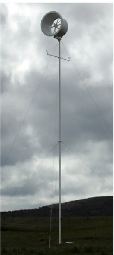
1.2 Enhanced WT prototype tested at 12 meters in unbuilt environment. . . . 6
2.1 Actuator disk model of a wind turbine, adapted from (Jonkman 2003, Manwell et al. 2002). . . 10
2.2 Wake rotation structure (Jonkman 2003). . . 13
2.3 Theoretical maximum power coefficient as function of tip speed ratio for an ideal HAWT, with and without wake rotation, adapted from Eggleston & Stoddard (1987). . . 14
2.4 Theoretical power coefficients (CP) of wind rotors considering different designs as function of tip speed ratio (λ) (Wilson & Lissaman 1974, Hau 2006). . . 14
2.5 Schematic representation of systems that concentrate and accelerate the wind, adapted from Ohya et al. (2008). . . 15
2.6 Representative illustration of the flow around the shroud, considering the presence of brim, adapted from Ohya & Karasudani (2010). . . 17
2.7 Resultant forces acting on an airfoil (Jonkman 2003). . . 18
2.8 Pressure distribution around an airfoil (Vennard et al. 1996). . . 19
2.9 Airfoil nomenclature (Anderson 2001). . . 19
2.10 Blade element model, divided intodrsection (Kulunk 2011). . . 20
2.11 Blade geometry (cross section) for analysis of blade element theory (Jonkman 2003). . . 21
3.1 Subsonic Wind Tunnel. . . 32
3.2 Aerodynamic models produced considering a different scaling factor. . . . 33
3.3 Wind turbine model used in experimental setup. . . 35
3.4 Electrical circuit diagram used to evaluate electric power generated. . . . 35
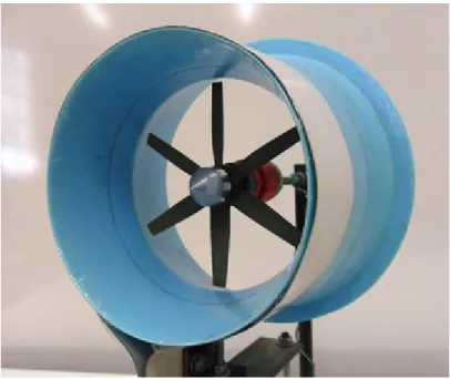
3.5 C-D system used in experimental trials. . . 36
3.6 Representation of the model developed by Paulo (2013), implemented in experimental wind tunnel setup. . . 36
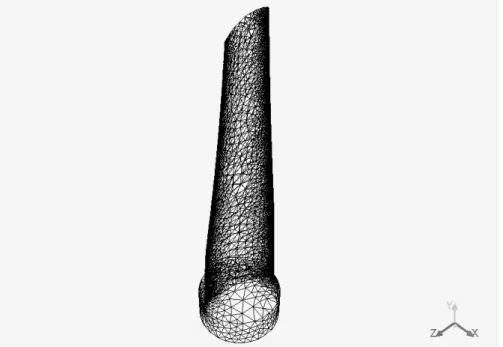
3.7 Mesh of blade computational domain, without the presence of virtual
wind tunnel structure. . . 38
3.8 Computational domain and boundary conditions. . . 39
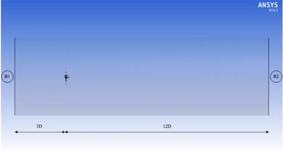
3.9 Computational domain produced with the enclosed wind turbine (B1 -velocity-inlet and B2 - pressure-outlet). . . 41
3.10 Computational domain specifications, WT distance relative to
velocity-inlet (B1) and with pressure-outlet (B2). . . 42
3.11 Computational mesh generated for the analysis of rotor performance. . . . 42
3.12 Computational domain produced with the enclosed C-D (B1 -
velocity-inlet and B2 - pressure-outlet). . . 43
3.13 Computational mesh performed for the analysis of effects that C-D
gen-erated in air flow. . . 44
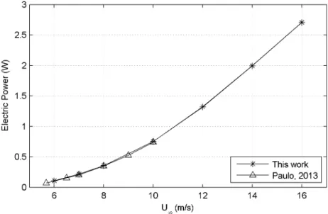
4.1 Experimental electric power generated by the aerodynamic model in wind tunnel trials. . . 50
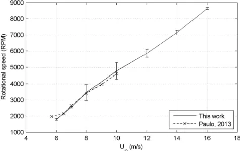
4.2 Errorbar graph of rotor rotational speeds obtained relative to those
de-scribed in Paulo (2013). . . 51
4.3 Wind Turbine power coefficient performance as function of different wind
speed values. . . 51
4.4 Experimental electric power generated by the implementation of shroud
in wind tunnel trials (△) compared to those described in Paulo (2013) (*) . 52
4.5 Electric power values in function of wind speed, in the case of Wind Tur-bine (*) and Wind TurTur-bine adapted with a Convergent-Diffuser (△). . . . 53 4.6 Evaluation of power coefficient performance performed to the Wind
Tur-bine (*) and Wind TurTur-bine comTur-bined with Concentrator-Diffuser (△) in function of wind speed values. . . 54
4.7 Computed Pressure Coefficient distributions on the aerodynamic model
blade 2. . . 56
4.8 Computed Pressure Coefficient distributions on the aerodynamic model
blade 1. . . 57
4.9 Blade surface turbulence kinetic energy plots overlaid with surface
stream-lines, for blade model 2. . . 58 4.10 Blade surface turbulence kinetic energy plots overlaid with surface
stream-lines, for blade model 1. . . 59
4.11 Computed wind turbine power coefficient performance as function of
dif-ferent wind speed values. . . 61
4.12 Streamline of air flow velocity that surrounds C-D device, considering an
4.13 Streamline of air flow velocity that surrounds C-D device, considering an
approaching wind speed of 14 m/s. . . 62
4.14 Radial contour of velocity experienced at rotor acting zone in C-D device,
pondering an approaching wind of 6 m/s. . . 63 4.15 Radial contour of velocity experienced at rotor acting zone in C-D device,
pondering an approaching wind of 14 m/s. . . 63
4.16 Turbulence generated at C-D outflow, evaluated in terms of turbulence
kinetic energy, considering an approaching wind of 6 m/s. . . 64
4.17 Turbulence generated at C-D outflow, evaluated in terms of turbulence
kinetic energy, considering an approaching wind of 14 m/s. . . 64
4.18 Drag force relative to the aerodynamic blade model 1 in function of attack
angle variation. . . 65
4.19 Lift force relative to the aerodynamic blade model 1 in function of attack angle variation. . . 66
4.20 Drag force relative to the aerodynamic model blade 2 in function of attack
angle variation. . . 67
4.21 Lift force relative to the aerodynamic blade model 2 in function of attack
angle variation. . . 68
4.22 Power coefficient confrontation through experimental (△) and numerical
3.1 Main dimensions on the C-D model design (Paulo 2013). . . 37
3.2 Sizing Mesh details applied on generation grid for models blade. . . 38
3.3 Boundary Conditions. . . 39
3.4 Optimal angular speed that rotor generates. . . 45
3.5 Methods applied in spatial discretization solutions. . . 45
4.1 Drag and lift force values (N) obtained in the evaluation of aerodynamic blade model 1. . . 48
4.2 Drag force and lift force values (N) obtained in the evaluation of aerody-namic blade model 2. . . 49
4.3 Comparison of electric power production data in function of wind speed values obtained for both situations. . . 53
4.4 Comparison of power coefficient data in function of wind speed values obtained for both situations. . . 55
4.5 Computed wind turbine torque as a function of the wind speed values. . . 60
4.6 Comparison between experimental torque data attained with the numeri-cal torque values in function of wind speed values. . . 69
C-D Concentrator-Diffuser
CAD Computer-Aided Design
CFD Computational Fluid Dynamics
DAWT Diffuser Augmented Wind Turbine
DNS Direct Numerical Simulations
HAWT Horizontal Axis Wind Turbines
IGES Initial Graphics Exchange Specification
MUSCL Monotone Upstream-Centered Schemes for Conservation Laws
RANS Reynolds-Averaged Navier-Stokes
SIMPLE Semi-Implicit Method for Pressure-Linked Equations
SIMPLEC Semi-Implicit Method for Pressure-Linked Equations Consistent
SRS Scale-Resolving-Simulation
UWT Urban Wind Turbines
WT Wind Turbine
Introduction
1.1
Motivation and Objectives
Large spread of wind technologies around the world has followed the constant increment
on energy consumption. Urbanized areas are large consuming centers and where
inte-gration of designed Urban Wind Turbines, UWT, could be encouraged. Wind energy in urban environment shown some sustainable energy potential for exploitation.
Day by day electricity becomes a decisive factor on the growth of economics and
sustainable development. Thus, associated with the increasing need for electrical power,
synergies with best practices should be established for it’s production. Linked to the
decentralization of energy production, it became possible an approach of electric power
producers elements with major consumption centers. Therefore, efforts to increase of
energetic wind turbine performance should be made, and small wind turbines should be
considered as part of the solution. These equipment’s must accommodate increase in
their energy performance, such that small energy gains, would contribute more to the sustainable development.
In this work, improvements on the energy production of small wind turbines (WT)
were studied. These improvements were obtained placing the rotor inside a C-D, designed
to accelerate the wind mass flow that pass through the rotor. Moreover, contributions on
the experimental and numerical simulations were produced, in order to verify enhance
that C-D produces in wind turbine production. C-D implementation verifies significant
considerations that would become a designed aerodynamic device that hereafter, will be
able to exploit the high potential exploitation present in the urbanized areas.
1.2
State of the Art
During the last years, significant progress has been made to understand the diffuser
tech-nology. Thus, new ideas have emerged on the origin of those technologies due to the
potential increase in efficiency that diffuser devices produce in wind turbines, particularly
for small wind turbines.
Numerous investigations relative to Diffuser Augmented Wind Turbine, DAWT, or
shrouded wind turbines concept over the last century were done.
As reported by Ten Hoopen (2009), Betz (1929) was the first to acknowledged the
potential of ducted / diffuser wind turbines. The idea of DAWT in a preliminary study
were proposed again by Lilley et al. (1956). The work from Lilley et al. (1956) the
increase in axial velocity and reduction of blade tip losses was described as been as the
main factors to enhance the power. A creation of a flow augmentation was also suggested,
where laying of a flap at diffuser exit plane would raise the power augmentation.
As described by Phillips (2003), Lilley et al. (1956) regarded the cost of ducted
wind-mill energy devices and suggested that one enhance of gain in power of at least 65 %
relative to conventional wind turbines is achievable.
Analyzing different shrouded rotors, Kogan & Seginer (1963) concluded that the
de-sign is one of the main factors to obtain a power augmentation. Nevertheless, they
sug-gested that the size of the duct become a commercially uncompetitive design.
Further-more, some serious flow separation inside the diffuser were described.
Experimental studies performed by Gilbert & Foreman (1983, 1979) and Igra (1981),
shown that power extraction beyond Betz limit is possible. Furthermore, DAWT
technol-ogy have been considered not profitable relatively to conventional wind turbines.
There-fore, these investigations were not continued.
In the case of Igra (1981) work, the power enhanced of a shrouded wind turbine is described as been as a direct consequence of the sub-atmospheric pressure created around
the rotor and at the exist plane of the diffuser. These sub-atmospheric pressures generate
one effect of suction that produces a higher mass flow.
Several maximum power coefficient values were reported and different mechanisms
that governing DAWT augmentation phenomena were proposed. The work from de Vries
(1979) stated that DAWT power augmentation is ruled by the force that simple diffuser
exerts on the flow. Furthermore, one analytical approach was made, based on work
devel-oped by Igra (1981), verifying in a maximum power coefficient of 0.7698.
Relative to renewed interest in DAWTs, an increasing number of publications have
been released and several attempts has been made to commercialize the idea.
The DAWT design and performance was optimized by Phillips (2003), applying CFD
methods, in which the wind turbine was modeled as an actuator disk. Also several small
scale experiments were developed. Phillips (2003) concluded that the data of the
full-scale DAWT shown only an augmentation of 2.4 instead of the expected 9, described in
other publications.
Recently, according some authors, a shaped diffuser structure involving the wind
of the diffuser.
Bet & Grassmann (2003) developed a shrouded wind turbine with a wing-profile ring
structure. An increase in power output by the wing system of 2.0 was obtained.
Addition-ally, Grassmann et al. (2003) continue the work performing some experimental measure-ments using a non-optimized wind turbine. The increase of power output in a factor of 55
% for high wind speeds and 100 % at low wind speed was described.
Wang et al. (2008) investigated convergent-divergent scoop effect on the power output
applying on small wind turbine. Results shown that the scoop increases the airflow speed
and enhance the power output 2.2 times relative to conventional wind turbines. These
results also indicate that electricity yield can be improved at lower wind speeds.
On Ohya & Karasudani (2010) a remarkable increase, in the output power of
approx-imately 4-5 times relative to conventional wind turbine is described. This, significant
increment, is induced by the low-pressure region, that generates a zone of strong vortex formation behind the broad brim that draws more airflow to the wind turbine inside the
diffuser.
Kosasih & Tondelli (2012) performed experimental studies of shrouded micro wind
turbines. Experimental measurements of coefficient performance shown an increase of 60
% in addition of a simple conical diffuser, and 63 % with the addition of nozzle - conical
diffuser shroud compared to the performance standard small wind turbines. Furthermore,
it’s described how the diffuser length and brim height can affect the performance
augmen-tation of micro wind turbines.
As described in Jafari & Kosasih (2014) diffuser generates a sub-atmospheric region at downwind, which seems to attract more wind through the rotor relative to a conventional
wind turbine. The work from Van Bussel (2007) showed that power augmentation is
related to mass flow augmentation which is performed by increase of the exit area ratio
and decrease of back pressure.
With modern computing power, more CFD studies have been performed on DAWT
including blade and shroud design.
Applying numerical simulations and Particle-Image-Velocimetry in wind tunnel
ex-periments Kardous et al. (2013) concluded that the utilization of a diffuser with a flange
is responsible of a wind speed increase rate ranged from 64 % to 81 % while diffuser
without flange is responsible only a increase rate of 68 %.
Toshimitsu et al. (2008) performed flow velocity measurements with flanged diffuser
by Particle-Image-Velocimetry. Results shown that turbine blades rotating effects
sup-press the turbulence and the flow separation near the inner diffuser surface. At diffuser
downstream some vortices, was consistently found such as, one behind the flange acts
suction effect on wind to the diffuser, consequently raise the inlet flow velocity. Hence,
diffuser device enhance the wind power in 2.6 times relative to standard wind turbine.
turbine configurations, and a low ratio between shroud radius to shroud chord length of the
diffuser is desirable, this indicate that the benefit of introducing shroud to a wind turbine is
more easily to realize in small wind turbines, where this ratio is feasible. Likely verified in
previous works, the shroud can be used effectively at low cut-in speeds and offers improve on the energy capture. Augmentation ratio of up to 1.9 with the introduction of a shroud
was obtained.
According with Mansour & Meskinkhoda (2014), CFD calculation was performed,
applying two different turbulence models for flow field around flanged diffuser. In short, a
remarkable increase in wind speed of 1.6-2.1 times higher compared to small wind turbine
was described. Furthermore, the turbulence models present the capability of providing
reasonable predictions for complex turbulent flows.
As previously mentioned the use of a diffuser induces flow separation, nevertheless as
seen in previous work flow separation can be suppressed. Extensive work from Gilbert & Foreman (1979) were made. The swirling flow produced by the rotor delays flow
separation inside the diffuser was concluded due to a momentum transfer to the boundary
layer.
Abe & Ohya (2004), Ohya & Karasudani (2010) have performed an extensive
experi-mental and numerical work that lead to the development of one high performance flanged
diffuser applied on small wind turbines. The pressure in the wake downstream of the
dif-fuser adding a flange around the trailing edge of the difdif-fuser, causing the flow to separate
and create a large low pressure region downstream of the diffuser creating a suction effect
through the diffuser was generated.
According with Shives & Crawford (2010) the flow separation of the boundary layer
in diffuser sections leads to significant loses in performance of DAWT. Nevertheless, the
base pressure effect provides a considerable enhancement.
Takahashi et al. (2012) worked on development of Wind-Lens turbine. The induced
vortex formed, probably by blade tip vortex within the boundary layer of the inner surface
of the diffuser, suppresses the flow separation from the inner diffuser surface. As result
collection and acceleration of the wind is augmented.
Jafari & Kosasih (2014) reported that flow separation in diffuser may lead to reduces
on overall power coefficient. This phenomenon can be mitigated by adapting the length
of the diffuser.
A new version of the classic Betz limit has been proposed by Jamieson (2008), which
describe that the maximum power extracted from a wind turbine with augmentation is
0.89 of the available power.
Recently, some methods to analyze the DAWT have been proposed. Vaz et al. (2014)
proposed innovative 1D mathematical model approach to the analysis of DAWT using
Blade Element Momentum model. Carroll (2014) creates one similar method to the way
axisym-metric surface vorticity method. It’s clear that these preliminary studies need validation
studies.
In short, DAWT configuration has received several evolutions on the understanding
of the phenomena that governing the effect that enhances the wind turbine production with a shroud device. However, all of this knowledge acquired, not led to any
commer-cial success so far by any company. Also, no commercommer-cial DAWT design tools have been
developed so far and it seems that the scientific community still has to agree on the
phe-nomena that govern the DAWT applications.
Concerning to this work, Enhanced Wind Turbine project has emerged from the work
developed by Paulo (2013).
Main idea ofEnhanced WTis enhance the productivity of urban wind turbines. There-fore, enhanced is achieved by encapsulating the wind turbine, accelerating the air flow
and thus creating more electric energy. Previous work developed by Ribeiro et al. (2013) describe that Enhanced WT shows a yield 120 % higher than the small wind turbines conventional models.
Enhanced WT is composed by a convergent - diffuser and a wind turbine, as can be seen in following Figure.
Figure 1.1: Schematic system representation composed by a concentrator-diffuser (C-D) and a wind turbine (WT), developed by Paulo (2013).
Also, at diffuser exit plane is accommodated a brim/flange, in order to exploit the
suction effect.
Moreover, in the phase of creation of the encapsulated parts of the structure
sustain-able materials are used. Materials like cork base products are integrated in the equipment.
Due to the potential application in urban environments this equipment have a positive
approach to urban space and the user. Moreover, initially enviable locations, low wind speeds or proximity of structures will become a favorable local to it’s installation.
and optimization of a shroud device for acceleration the wind to increase power in a wind
turbine were performed. Through numerical simulations, one medium power increase of
71 % was obtained relative to standard wind turbine. Nevertheless, are verified higher
values in the case of wind tunnel measurements. Therefore, the medium power increase of 107 % was obtained.
According with García-Abril (2014), numerical studies were performed for enhance
the performance, optimizing the diffuser outlet angle. Despite of several angle have been
studied, the 25º (without roughness) and 27º (with roughness) was considered those that
enhance the power. These models suggest an improvement of 3.6 % to 8.7 % relative to a
initial model (20º). As noted previously this study also concluded that the use of shrouded
rotors induce a suction effect due to a pressure gradient generated in outlet of C-D.
Associated with the development and investigation of the research projectEnhanced WT was created and tested a prototype, as can been seen from Figure 1.2. Presently, this project is in final prototype phase and soon pre-industrial series will accommodate some
progress.
1.3
Structure
The fundamental motivations of this work are presented in Chapter 1, along a literature
review on the shrouded wind turbines and a review ofEnhanced WTproject. In Chapter 2, the fundamentals concepts/theories of wind turbines aerodynamics are presented with the
main theoretical concepts of Computational Fluid Dynamics (CFD ). Chapter 3 is
dedi-cated to presentation of the several methodologies applied on experimental and numerical
tests. Chapter 4 includes a detailed analysis of the results obtained in the experiments and
in numerical simulations. Finally, in Chapter 5, the main conclusions and suggestions for
Literature Review
Along this chapter, is presented the main theories for the assessment of shrouded wind
tur-bines and for blade aerodynamics evaluation. Also are depicted several concepts related
to the Computational Fluid Dynamics component.
2.1
Wind Turbine Aerodynamics
The existence of accurate models of aerodynamics aspects of wind turbines is one key
point for a successful designing and analyzing wind energy systems. Wind turbines
operation induces phenomena like cross-flow components (when a rotor is not aligned with wind), where magnitude and direction relative to the rotor changes as the blades
rotate. Moreover, in these cases, phenomena like flow separation and three-dimensional
effects becomes significantly more complex. Those instabilities interacting with blade,
hub and tip form vortices that affect the character of the whole flow field. Clearly, wind
turbine aerodynamics becomes more complex with all instabilities and flow interactions
(Jonkman 2003).
Firstly, to understand the complex physics involving wind turbine aerodynamics, one
should analyze a simple one-dimensional model.
The following sections were performed for an incompressible fluid. According with literature the flow velocity is a factor that determines the compressible or incompressible
of the flow. Usually, as the blade tip speed do not exceeded 100 m/s which is equally to an
Mach number of 0.3, and thus the flow around the rotor is assumed to be incompressible
(Schlichting 1979).
2.1.1
Actuator Disc Model and Betz Limit
The simplest one-dimensional wind turbine model is so-called as actuator disc model
where the turbine is replaced by a circular disc through which the flow streamlines passes with a velocity,U∞.
The following equations presented in this section were based from Wilson & Lissaman
(1974), Jonkman (2003), Manwell et al. (2002), Kulunk (2011).
The analysis assumes a control volume and are need to considers some assumptions:
Wind is steady, homogeneous and have a fixed direction; air is incompressible, inviscid; an infinite number of blades need to be considered; a non rotating wake is considered;
uniform thrust over the rotor needs to be assumed and the static pressure far upstream and
far downstream of the rotor is equal to the undisturbed ambient.
A simple schematic of this control volume is shown in Figure 2.1.
Figure 2.1: Actuator disk model of a wind turbine, adapted from (Jonkman 2003, Manwell et al. 2002).
In order to study this control volume, four regions (Figure 2.1) need to be considered
as: 1: free-stream region; 2: before rotor; 3: after rotor and 4: far wake region. In
free-stream region is assumed thatU∞=U1.
Applying the conservation of linear momentum to the control volume, and considering
a steady-state flow, the thrust is equal to:
T =m˙(U1−U4) (2.1)
where, ˙mis the mass flow rate, and is equal to ˙m= (ρAU)1= (ρAU)4, representing, ρ, air density,Athe cross sectional area and,U, the air velocity.
The thrust is positive so the velocity behind the rotor,U4, is lower than theU1.
Since the flow is frictionless and there is no work or energy transfer is done, Bernoulli
equation can be applied on both sides of the rotor.
p1+ 1 2ρU
2
1 = p2+ 1 2ρU
2
2 (2.2)
p3+ 1 2ρU
2
3 = p4+ 1 2ρU
2
4 (2.3)
(p1= p4)and the velocity across the rotor stays equal (U2=U3).
The thrust on the rotor disk,T, is also the differential pressure between stations 2 and 3 multiplied by the disc area:
T =A2(p2−p3) (2.4)
Using Equations 2.2 and 2.3 and substitutes that into Equation 2.4 is obtained:
T = 1
2ρA2(U 2
1−U42) (2.5)
Recognizing now that ˙m=A2U2 and equating the thrust Equations 2.1 and 2.5, are obtained:
U2=
U1+U4
2 (2.6)
Thus, the wind velocity at rotor plane, is the average of the upstream and downstream
wind speeds.
An axial induction (or interference) factor,a, measures the influence of the wind being slowed down as result of power extraction by the rotor. It’s defined as the fractional
decrease in wind velocity between the free stream and the rotor plane:
a=U1−U2
U1
(2.7)
U2=U1(1−a) (2.8)
U4=U1(1−2a) (2.9)
The power extracted from the wind by the rotor,P, is the product of the thrust,T, and the wind velocity at the rotor plane,U2.
P=TU2 (2.10)
P= 1
2ρA2(U 2
1−U42)U2= 1
2ρA2U2(U1+U4)(U1−U4) (2.11) Substituting forU2andU4from Equations 2.8 and 2.9 gives:
P= 1
2ρAU 34a(1
−a)2 (2.12)
where the control volume, A2, is replaced with A, the rotor area, and the free stream velocityU1is replaced byU.
representing the fraction of available power in wind that is extracted by the turbine, is
defined as:
CP=
P
1 2ρAU3
(2.13)
Substituting the extracted power form Equation 2.12 into Equation 2.13:
CP=4a(1−a)2 (2.14)
The theoretical maximum power coefficient from an idealized rotor,CPmax, known as
Betz limit, can be found by setting the following derivative with respect toaequal to zero, and solving fora:
∂CP
∂a =4(1−3a
2) =0
⇄a= 1
3 (2.15)
Substituting into Equation 2.14, yielding:
CPmax=
16
27 ≈0.59259 (2.16)
For an idealized wind turbine, the maximum efficiency is equal to 59.3 %. In practice, some considerations can be listed for real wind turbines do not present this efficiency:
Rotation of the wake caused by the rotor; finite numbers of blades; viscid flow causes
nonzero aerodynamics drag.
2.1.2
Effects of Wake Rotation on Betz Limit
Wakes behind Horizontal Axis Wind Turbines, HAWT, are a complex turbulent flow
structures with rotational motion induced by the turbine blades movement, pressure slopes
and tip vortices (Mo et al. 2013).
Two type of characteristics of wind turbine wakes can be enumerated: the velocity
deficit, which is related to the power loss from wind turbine and turbulence levels, which
may affect aerodynamic performance of other turbines located at downwind.
Understand-ing these effects is among the main reason why turbines wakes have been subjected to a
consistent research (Chamorro & Porté-Agel 2009).
Moreover, a clear analysis of these effects in consideration of Betz limit proves to be
an important consideration for the study of aerodynamic performance of HAWT.
The previous analysis can be extended to the case with rotating rotor generates angular
momentum, having relationship with rotor torque. The flow behind rotor have an opposite rotation direction relative to wind turbine rotor. Present reaction is caused by the torque
exerted by the flow on the rotor. Figure 2.2 shows an example wake rotation generated by
Figure 2.2: Wake rotation structure (Jonkman 2003).
The generation of rotational kinetic energy in the wake produces a lower energy
ex-traction by the rotor that would be expected without wake rotation. Thus, with increasing
of torque generation therefore will be also verified a higher production of the kinetic
en-ergy in the wind turbine wake.
Following a procedure similar to that used in section 2.1.1, accounting with wake
rota-tion those equarota-tions can be used to modify the theoretical maximum power coefficient for
an idealized rotor,CPmax. According with the work developed by Eggleston & Stoddard
(1987), values of theoretical maximum power coefficient where obtained considering the wake rotation phenomena.
It’s worth noticing that, the work developed by Eggleston & Stoddard (1987) evaluates
the maximum power coefficient as function of the tip speed ratio. The tip speed ratio,λ, is defined as the ratio of the blade tip speed to the free stream wind speed and is calculated
as:
λ = ΩR
U∞ (2.17)
where,Ω, is angular velocity and,R, is the radius of turbine blades.
Figure 2.3: Theoretical maximum power coefficient as function of tip speed ratio for an ideal HAWT, with and without wake rotation, adapted from Eggleston & Stoddard (1987).
Extending this analysis to different wind turbine types an identical evaluation of power
coefficient as function of tip speed ratio can be performed. Thus, in following Figure 2.4
is described that evaluation.
Figure 2.4: Theoretical power coefficients (CP) of wind rotors considering different
In Figure 2.4 are presented power coefficients performances of rotors that presents
different configurations. Nevertheless, is emphasized the performance curve of American
Wind Turbine, due to this configuration be considered similar to the studied in this work.
From all the configurations described in Figure 2.4, it appears that the American Wind Turbine, describing 8 blades, displays a configuration closest to the used in this work,
which features 6 blades.
2.1.3
Theoretical Analysis of Shrouded Rotor
In order to evaluate concepts like shrouded rotors is prudent to examine the theoretical
background which governing performance of shrouded rotors.
According with augmentation ratio,ra, is possible to describe the enhance power
ex-tracted from a wind turbine combined with a diffuser. Therefore, augmentation ratio is
defined as (Aranake et al. 2013):
ra=
CP,d
0.593 (2.18)
whereCP,dis power coefficient for a wind turbine with diffuser.
Shrouded rotors can combine different systems in order to help to concentrate and
accelerate the wind. Hollow structures can be applied for surrounding a wind turbine to
enhance the wind flow. As can been seen in Figure 2.5 nozzle model section reduces the
inside cross-section, in cylindrical model section may have a constant cross-section, and
diffuser model section have cross-section at downstream that expands (Ohya et al. 2008).
Figure 2.5: Schematic representation of systems that concentrate and accelerate the wind, adapted from Ohya et al. (2008).
Applying nozzle, with converging shape, at inlet of shrouded wind turbine, will
be-come beneficial mainly in variable wind direction flow condition, which is typical in urban scenario (Kosasih & Tondelli 2012).
The shrouded rotors exploit the Venturi effect, where the reduction of fluid pressure
and the associated elevation of fluid velocity, are produced by the passage of a flow in
a contraction. For a shrouded rotor, the contraction is performed by the shroud that
sur-rounding the rotor (Hjort & Larsen 2014). At nozzle section, the inlet diameter is larger
it comes to the outlet, the velocity gets increased due to the reduction of area (Balaji &
Gnanambal 2014).
The principle of increase the mass flow through the wind turbine can be combined
with the turbulent mixing of the wake behind the rotor providing a power augmentation (Ten Hoopen 2009).
It’s well proven that when a bare wind turbine is operating at the maximum Betz limit,
the airflow is decelerated to2/3of the free stream velocity. This flow deceleration causes
a pressure increase in front of the rotor that induces a small portion of the mass flow being
pushed sideways around the rotor (Ten Hoopen 2009).
A mechanism to increase air flow can be applied placing an annular lifting device
around the rotor. This device is known as a shroud or a diffuser of annular wing. The
increase in diffuser exit plane velocities combined with a reduction of static exit pressure
and consequently is obtained an enhanced of mass flow leading to a higher extraction of energy potential. The principle behind a DAWT can be assumed as the cause of the air
flow on the inside the diffuser to accelerate. Furthermore, the suction is related to the lift
of the airfoil and according to the Kutta Joukowski theorem, related to the bound vorticity.
The annular airfoil generates a radial lift force creating a ring vortex, based on Bio-Savart
law, that consequently will induce a higher velocity on the suction side. Furthermore, this
higher velocity enhance the mass flow through the rotor plane (Ten Hoopen 2009).
Associated at energy extraction from an air flow a wake behind the rotor is produced.
This wake has a pressure and a velocity deficit relative to undisturbed free stream flow.
According with (Igra 1981, Van Bussel 2007), the power augmentation of a DAWT is a direct consequence of the sub-atmospheric pressure around the rotor and exit plane of the
shroud.
DAWT configuration allows tip vortices created at the blade tips to be significantly
less due to close proximity of the diffuser wall. Therefore, mixing potential behind the
exit plane of a DAWT is expected to be higher than in the case of conventional wind
turbine (Ten Hoopen 2009).
The mixing of effect on diffuser leeward provides one wake flow with more volume.
Furthermore, a larger wake volume will induce lower exit pressures behind the rotor and
therefore more suction effects (Ten Hoopen 2009).
In order to take advantage of mixing effects flanged applications on shroud plays an important role. This flanged, also known as brim, collects and accelerates the approaching
wind (Ohya et al. 2008). The flanged is placed at the exit plane of the shroud, such as in
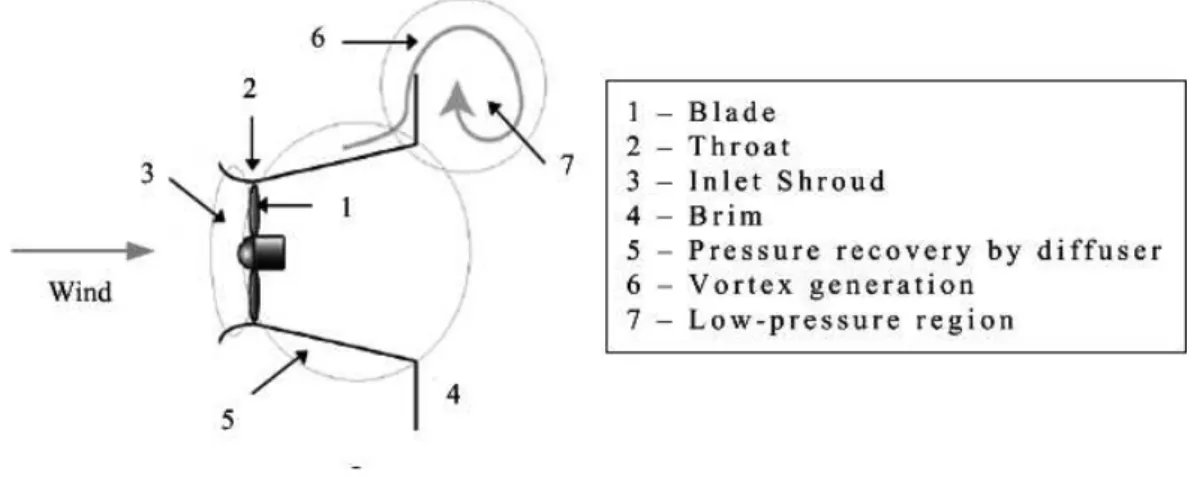
Figure 2.6: Representative illustration of the flow around the shroud, considering the presence of brim, adapted from Ohya & Karasudani (2010).
The flange is a structure ring-type plane with a variable height may affect the shroud
performance. It’s placed attached vertically to the outer periphery of exit shroud (Ohya
et al. 2008, Kosasih & Tondelli 2012).
As can be seen from Figure 2.6, the flange induces a low-pressure region in the near
wake of the diffuser by vortex generation. Furthermore, more mass flow is drawn to the
inside of shroud (Ohya et al. 2008, Ohya & Karasudani 2010, Takahashi et al. 2012). The
flange causes vortices formation, an enhancer in the pressure drop and, consequently, an
increase the air speed of the outlet. An increase the air velocity in the diffuser, is therefore,
achieved (Mansour & Meskinkhoda 2014).
In Figure 2.6, the “throat” plane represent the diffuser cross section perpendicular to
the axisymmetric axis where the area inside the diffuser is smallest (Hjort & Larsen 2014).
An important characteristic can be described from the application on a brimmed dif-fuser shroud. Brim application helps the shroud, for automatically, stay aligned to the
approaching wind. Another characteristic verified at low-tip speed ratio range that vortex
generated from blade tip becomes suppressed through the interference with the boundary
layer within the diffuser shroud. Therefore, aerodynamic noise is substantially reduced
(Abe et al. 2006, Ohya & Karasudani 2010).
2.1.4
Forces Acting on a Blades
Mainly can be shown two examples of manifestation the main forces in wind turbine operation. Expression of drag force can be evidenced when a wind turbine presence high
wind and is stationary where the primary consideration is the drag force. In contrast, when
a wind turbine is operating it’s lift force, produced by blades, which create aerodynamic
loading and consequently is generated mechanical energy (Burton et al. 2001, Manwell
et al. 2002).
field downstream of the object will be asymmetric and the velocity and pressure
down-stream and updown-stream will be different. Consequently a normal force to flow will generated
in object. The same behavior is verified for objects whose axis isn’t perfectly aligned.
Therefore, is expected that the action of friction tension will produce a resultant force pair in opposite direction of flow due to boundary layers of surface body. Thus, this force
is opposed to motion of body (Vennard et al. 1996).
In short, the pressures and friction tensions produce a resultant force pair
perpendic-ular between themselves designed by drag and lift. Therefore, the drag produced by flow
around an object is defined as the forces that act on body in the parallel direction to flow
direction. Relatively to lift is defined like a force that act on body in a normal direction to
flow direction (Burton et al. 2001, Vennard et al. 1996). These characteristics are depicted
in following Figure 2.7.
Figure 2.7: Resultant forces acting on an airfoil (Jonkman 2003).
An effective moment results of these forces. Thus, usually is defined about on normal
axis to the cross-section of the airfoil, located at quarter of the distance from the leading
edge to the trailing edge (Jonkman 2003).
The forces acting on an object by a flow are due to pressure and viscous stresses. On
the upper surface of an airfoil, the pressure is less than that of the flow stream which sucks
the airfoil upward, normal to the incoming flow. On the other hand, the pressure on the
lower surface of the airfoil is greater than that of the flow stream and effectively pushes
the airfoil upward. Due to this, pressure distribution component tends to slow the velocity of the incoming flow relative to the airfoil, as well as viscous stresses (Jonkman 2003).
Figure 2.8: Pressure distribution around an airfoil (Vennard et al. 1996).
The pressure distribution of both sides of the airfoil, present on Figure 2.8, have a
positive contributions to lift generation. By contrast, the viscous stresses have a negligible contribution to the lift force. The part of the drag force related to pressure distribution
around the airfoil is classified as pressure drag. Thus, the part relative to viscous stresses
is known as skin-friction drag. Sum of both perform total drag force, defined as drag
(Jonkman 2003).
The drag force,FD, and lift force,FL,are defined respectively as:
FD=
1
2×ρ×CD×A×U 2
∞ (2.19)
FL =
1
2×ρ×CL×A×U 2
∞ (2.20)
whereCL andCD are lift coefficient and drag coefficient, respectively and, A, represents
blade area.
2.1.5
Airfoils
Airfoils, presents a well-designed form projected for integration on many areas such as
wind blades conception (Chen 2011). Some terms usually are used for characterization
of this structure, which are represent on Figure 2.9.
An airfoil, presents divided by the mean chamber line, which define the locus of points
halfway between lower and upper surface. In most forward and rear points of this line
are contained the leading and trailing edge, respectively. The line how connect leading
and trailing edge is classified as chord line, and that distance measured in this line is designated as chord, c. The thickness is measured perpendicular to chord line, and is the distance among lower and upper surface. The chamber is represented as the distance
between chamber line and chord line, also valued perpendicular to chord line (Manwell
et al. 2002). At last, attack angle,α, if defined as the angle form between chord line and the relative flow.
In conception of wind turbine blades are regarded different shapes of airfoil along the
cross-section of the blade. Along the length are verified different values of thickness.
Thus, the blade tip is designed using a thin airfoil, for obtain a high lift to drag ratio.
By contrast, root region is designed using a thick version of one airfoil to obtain strength important for structural support (Manwell et al. 2002).
2.1.6
Blade Element Theory
Blade element theory refers to an analysis of forces at a section of the blade, as a function
of blade geometry. Following Figure 2.10 describes the blade divisions intodrsection.
Figure 2.10: Blade element model, divided intodrsection (Kulunk 2011).
Additional equations concerning the state of flow need to be developed. The state of
flow governed by characteristics of rotor blades needs to use the blade geometry properties
to determine the forces exerted on a wind turbine by the flow stream. This type of analysis
is referred to as Blade Element Theory.
At each section blade and flow stream properties can be assumed differential rotor
thrust, dT, and differential rotor torque,dQ. For this consideration certain assumptions needs to be made (Manwell et al. 2002):
• The forces that acts on the blades are set exclusively by the drag and lift
character-istics of the airfoil shape.
The differential rotor thrust,dT, and differential rotor torque, dQ, acting on each blade section as described by blade element theory is represented on Figure 2.11.
Figure 2.11: Blade geometry (cross section) for analysis of blade element theory (Jonkman 2003).
were,θPis the blade collective pitch angle measured relative to the point of zero twist,
θT is the local blade twist angle andθPT is their sum.
Note also, that angleθ is the angle of the relative incoming flow stream with respect to the plane of rotation and is equal to the sum ofθPT andα (Jonkman 2003).
The velocity of the incoming flow relative to the blade element geometry,U∞, is the vector sum of the axial inflow velocity at the rotor plane,U, the inflow velocity caused by the rotation of the blade,Ωr, and the inflow velocity caused by wake rotation at the rotor plane,ωr(Jonkman 2003).
U=U0(1−a) (2.21)
ω =Ωa′ (2.22)
U∞= q
[U0(1−a)]2+ [Ωr(1+a′)]2 (2.23)
Also relation betweena,a′, andθ can be developed:
tan(θ) = U0(1−a)
Ωr(1+a′) (2.24)
Regarding the resultant forces some relationships can be extracted from Figure 2.11 (Jonkman 2003, Manwell et al. 2002):
FL=
1 2CLρU
2
∞cdr (2.25)
FD=
1 2CDρU
2
∞cdr (2.26)
where,c, represents chord dimension.
dT =FL×cos(θ) +FD×sin(θ) (2.27)
dQ=r[FL×sin(θ)−FD×cos(θ)] (2.28)
If the rotor hasBblades, the differential rotor thrust,dT, and differential rotor torque,
dQare to following:
dT = 1
2BρU 2
∞[CLcos(θ) +CDsin(θ)]cdr (2.29)
dQ= 1
2BρU 2
∞[CLsin(θ)−CDcos(θ)]crdr (2.30)
dT and dQ represents the total differential thrust and differential torque, respectively, acting on an annular ring of radiusr and thicknessdr. It’s worth noticing, that the effect of drag force is to decrease torque and hence power, but to increase the thrust loading
(Manwell et al. 2002).
Momentum theory uses a control volume analysis to study the forces at the blade based on the conservation of linear and angular momentum. Blade element theory refers
to an analysis of forces at a section of the blade. The results of these theories can be
combined and form a theory designed as blade element momentum (BEM) theory.
2.2
Numerical Simulation (CFD)
Wind turbine design and aerodynamic performance are an important scientific field. In
op-timization to perform an upgrade on energy production of wind turbine (Lanzafame et al.
2013).
Computational fluid dynamics consists of solving the Navier-Stokes equations with
governing fluid flow using approximation with numerical means (Sumner et al. 2010). CFD solvers are based on following three fundamental conservations principles expressed
in terms of mathematical equations: Conservations mass; conservation of momentum and
conservation of energy (Sargsyan 2010).
In Versteeg & Malalasekera (2007) is described that one of the fundamental task of
the CFD user have is to design a grid that presents a suitable compromise between desired
accuracy and solution cost. Another concerning in the numerical simulations
simultane-ously are moving and stationary components that exist, which must be handled separately
(Bazilevs et al. 2011).
Extensive implementation of numerical simulations in aerodynamic features, applied on different manners, ranging from Blade Element Momentum methods integrated by
CFD solver to full 3D Navier-Stokes models became an important manner to evaluate
wind turbines performance (Sargsyan 2010).
Performing CFD calculations provide endless details knowledge of the fluid flow, such
as velocities, pressure, temperature, turbulence, etc. Further, several type graphics are
possible to obtain, performing results in flow lines, contour lines and iso-lines, etc. At
this stage, is assumed by Castelli et al. (2013) that these results can be compared to that
obtained in a wind-tunnel study or an elaborate full-scale measurement campaign.
3D CFD numerical codes are physically realistic, due to solve the Navier-Stokes equa-tions. Nevertheless, to achieve these solutions longer computational times are needed.
Also an accurate preparation of geometry is necessary. In spite of some problematic
is-sues that involves separated flow modeling globally CFD codes are an important mean
to achieve knowledge that are impossible to reach in experimental measurements
(Lan-zafame et al. 2013).
2.2.1
Governing Equations
The fluid dynamics involves complex relationships between the viscosity and how the
flow develops, translating into mathematical models induces a high level of complexity for some problems (Massey 1996).
The true fluid flow passing through and around a wind turbine is governed by the
main-principles of Navier-Stokes equations. Unfortunately, these equations are so complex that
analytical solutions only have been found for simple cases. Although numerical solutions
presents abilities to solve these equations (Jonkman 2003).
As shown by Trias & Lehmkuhl (2011) the incompressible Navier-Stokes equations
are a set of partial differential equations that translate to a unit volume of fluid flow, a
balance between the product of it’s mass and the corresponding acceleration (Oliveira &
Lopes 2012).
Major CFD models are based on the incompressible Reynolds-Averaged Navier-Stokes (RANS) equations derived from the main principles of conservation of mass and
momen-tum Sumner et al. (2010):
∇−→U =0 (2.31)
∂−→U
∂t +∇
−
→U =−1
ρ∇p+∇τ+ −
→f (2.32)
where,−→U represents the mean velocity vector, pis the modified mean pressure,ρ is the fluid density,−→f represents a body force andτperform the specific Reynolds stress tensor.
2.2.2
Structure of CFD Code
CFD codes are constructed around numerical algorithms that are developed for resolution
of fluid flow problems. Aiming to provide intuitive tools for users of complex CFD codes, normally these are divided in three elements: (i) Pre-processor, (ii) Solver, (iii)
Post-processor (Versteeg & Malalasekera 2007).
The pre-processor phase consists in the introduction of physical flow model with the
intention of converting in a mathematical model (Sargsyan 2010). The principles activities
of user’s are: definition of computational domain; grid generation of problem; modeling
of physical/chemical phenomena (e.g. turbulence models, radiative heat transfer,
com-bustion models); definition and specification of fluid properties and boundary conditions
of cells which have relation with another boundary (Versteeg & Malalasekera 2007).
In general, the precision of solution obtained are governed by the number of cells in the grid. So larger the number of cells contained in grid domain, more accurate will be the
solution. In short, both precision of solution as the cost in terms of computer capacity and
calculation time are dependent on the grid excellence (Versteeg & Malalasekera 2007).
The principal element of CFD code is the solver. The core of CFD code works with
discretization of governing equations fluid flows. In this phase, are modeled the unknowns
and solved with a resolution of algebraic system of equations (Versteeg & Malalasekera
2007, Sargsyan 2010).
At last, post-processor phase analysis solution results. With the evolution of CFD
packages results in a number of ways of visualization of solver outputs. So it’s possible set graphs and contours, perform domain and grid visualizations, introduce vectorial plots
and path-lines, and to perform also dynamic representations using animations (Sargsyan
2.2.3
Grid Generation
In numerical simulation applied for areas as science and engineering a mesh generation
is often described being a fundamental pre-requisite. The growing of mesh generation
brought new ideas and ways of viewing mesh related issues (Baker 2005).
It’s well known that, approximately over 50 % of time spent in development of CFD projects is devoted to the definition of computational domain and grid generation
(Ver-steeg & Malalasekera 2007).
Furthermore, a compromise between number of cells/domain size and computational
time need to exist. Due to a consideration of one small domain would not provide enough
grid generation, while a too great domain would lead to an increasing of computational
time, that are unnecessary for certain cases (Lanzafame et al. 2013).
According to Baker (2005) grid generation has evolved to a point where complicated
domains can be covered by a variety of mesh types.
Several grid types can be classified as structured, unstructured and hybrid type. In short, structured grids are defined by their regular connectivity, that is not verified in
un-structured grids that presents an irregular connectivity between elements. Relatively to
hybrid grids, these type contain an efficient mixture of structured portions and
unstruc-tured portions (Baker 2005, Bern & Plassmann 2000).
A major applications of unstructured grid is verified in finite elements calculations
(Digraskar 2010).
The element quality and how this affect the solution accuracy is still a research area
that has some question unanswered (Baker 2005). As like as “mesh quality” definition,
that according to Knupp (2007) is defined as been as “the characteristics of a mesh that permit a particular numerical partial differential equation simulation to be efficiently
per-formed with fidelity to the underlying physics and with the accuracy required for the
problem”. Associated to meshes composed by complex geometries two fundamentals
is-sues can be described for the quality of a finite element mesh (Burkhart et al. 2013). The
first can be considered as the shape of the elements that are selected to generate the mesh.
Moreover, two element shapes (tetrahedral and hexahedral) for discretize the complex
ge-ometries are used. On the other hand, the coarseness of the mesh is also considered. In
other form, the number of elements that the mesh is composed. Thus, in literature can
be found that an optimal mesh density exists when is provided the most accurate solution
with the smallest number of elements (Burkhart et al. 2013).
2.2.4
Finite-Volume Method
Most of the commercial CFD codes are based on the method of a finite volume
discretiza-tion (Carcangiu 2008). The finite-volume method is responsible for sub divide the domain
are applied to those control volumes (Ferziger & Peric 2002). This method can
accommo-date any type of grid, so it’s suitable for complex geometries (Ferziger & Peric 2002). A
detailed description of the finite-volume method is presented in Ferziger & Peric (2002).
FLUENT uses a cell-centered finite-volume method based on multidimensional lin-ear reconstruction scheme. Allowing the use of computational elements with arbitrary
polyhedral topology (quadrilateral, hexahedral, triangular, tetrahedral, pyramidal,
pris-matic) (Mo et al. 2013). FLUENT also uses a control-volume-based technique to
re-model the governing flow equations into algebraic equations that can be solved
numeri-cally (Makridis & Chick 2013). This technique consists of integrating transport equation
in each volume, resulting in a discrete equation that expresses conservation laws based on
the logic of a closed control volume (Fleck 2012).
In short, control-volume technique used by FLUENT consists in: Division the
do-main into discrete control volume using a computational mesh; integration of the basic governing equation on the control volumes to produce algebraic equations for the
dis-crete variables and application of linearization of the discretized equations and solution
of the resultant equation system (Carcangiu 2008, Versteeg & Malalasekera 2007, Fluent
2011a).
In ANSYS FLUENT core are available two numerical methods, applied for several
conditions. Pressure-based solver were developed for low-speed incompressible flows.
Although, the second solver, designed as density-based solver, were created for
appli-cation in high-speed compressive flows. In present work, involves incompressible flows
clearly pressure-based approach was applied.
The pressure-based solver uses an algorithm that pertains to a group of methods
de-signed as projection method. In this method, the restriction of mass conservation of the
velocity field is achieved by solving a pressure equation. The pressure equation is derived
from the continuity and momentum equation in such a way that velocity field, corrected
by the pressure satisfies the continuity equation. The complete solution process involves
iterations wherein the entire groups of governing equations are solved repeatedly until the
solution converges (Fluent 2011b).
2.2.5
Turbulence Modeling
As previously stated in subsection 2.2.2, modulation of physical phenomena is one of the
main issues that the user must take into account. Moreover, in this work will be taken
into account the turbulence generated in problems of the fluid mechanics area. Therefore,
to understand the turbulence modulation it’s important firstly, to describe the Reynolds
number.
Re= L×U
ν (2.33)
where, L is the characteristic over a body dimension of the flow (m); U is the mean velocity (m/s); andν is the kinematic viscosity (m2/s).
The Navier-Stokes equations applied for model of turbulent flows, in some situations are impractical to resolve for some ranges of scales in Direct Numerical Simulations
(DNS) due to high requirements of computing power. Therefore, averaging procedures
need to be applied to Navier-Stokes equations to filter part of the turbulent spectrum. The
principal averaging procedure applied is Reynolds-averaging of the equations, which
re-sult in the Reynolds-Averaged Navier-Stokes (RANS) equations. In this procedure
turbu-lent structures are eliminated and it’s feasible to obtain a smooth variation of the averaged
velocity and pressure fields. However, RANS equations introduce additional unknown
terms into transport equations which are solved by turbulence model (Fluent 2011a). An alternative to RANS equations are Scale-Resolving-Simulation (SRS). In these methods, at least one section of the turbulent spectrum is solved in at least a part of
the flow domain. Comparative to RANS simulations, all SRS methods require
time-resolved simulations with small time steps. These methods also are considerably more
computationally expensive than RANS models (Fluent 2011a,b).
RANS models are the most economic approach for computing of complex turbulence
applications. Positively, RANS models are available for all range of applications
provid-ing a level of accuracy required. The most well-known models arek-ε andk-ω. These models contribute for simplify of the problem, adding two additional transport equations
and introduce a turbulent viscosity to solve the Reynolds Stresses (Fluent 2011a,b, 2005). The choice of turbulence model it’s an important step to make once affect all quality
of the simulations. For selection of turbulence model is necessary apply some
consider-ations such as, fluid behavior, the level of accuracy required, the available computational
resources, the time of simulation and provides a suitable numerical grid and the time spent
(Fluent 2011a).
2.2.5.1 k-ε Model
By definition, two equation models include two extra transport equations for represent
turbulent properties of the flow. For the case of k-❡models the first transported variable
is often turbulent kinetic energy,k, which define the energy present in turbulent flow. The second transported variable is turbulent dissipation, ε, and represent scale of turbulence (CFD-Wiki2005).
reason-able accuracy (Fluent 2011a).
The standard form of thek-ε turbulence model is originally proposed by Launder & Spalding (1972) . Thus, following equations are described inCFD-Wiki(2005), Fluent (2005), Wilcox (1994). The turbulent kinetic energy, k, and it’s dissipation rate, ε, are obtained from the following transport equations:
∂
∂t(ρk) +
∂k
∂xi
(ρkui) =
∂ ∂xj
(µ+ µt
σk) ∂k
∂xj
+Gk+Gb−ρε+Sk (2.34)
∂
∂t(ρε) +
∂ ∂xi
(ρεui) =
∂ ∂xj
µ+ µt
σε ∂ ε
∂xj
+C1ε
ε
k(Gk+C3εGb)−C2ερ
ε2
k +Sε
(2.35)
In these equations,Gk, represents the generation of turbulence kinetic energy due to
the mean velocity gradients, and is described in Fluent (2005). Gb is the generation o
turbulence kinetic energy due to buoyancy, calculated in Fluent (2005).C1ε,C2ε andC3ε
are constants, also σk and σε are turbulent Prandtl numbers for k and ε. Sk and Sε are
user-defined sources terms.
The turbulent/eddy viscosity(kg m−1s−1)is modeled as:
µt =ρCµ
k2
ε (2.36)
where the closure coefficients for standardk−ε model are:
C1ε =1.44, C2ε=1.92, C3ε =−0.33 Cµ=0.09, σk=1.0, σε =1.3 (2.37)
The use of Realizablek−ε models is recommended relative to other variants of this family models, combining with Enhanced Wall Treatment (Fluent 2011a).
The realizablek−εmodel proposed by Shih et al. (1995) differs from standard model in two important ways: The realizablek−εmodel contains a new formulation for the tur-bulent viscosity; and a new transport equation for the dissipation rate,ε, is proposed. New transport equation have been reached from derivation of an equation transport of
mean-square vorticity fluctuation. The terms “realizable” means that model satisfies “certain
mathematical” constraints on the Reynolds stresses (Fluent 2005).
Note that following set of equations are described in Fluent (2005), Shih et al. (1995),
Cabezón et al. (2011).
The modeled transport equations for the,kandε, in the realizablek−ε model are:
∂
∂t(ρk) +
∂k
∂xj
(ρkuj) =
∂ ∂xj
(µ+µt
σk
)∂k
∂xj
∂
∂t(ρε)+
∂ ∂xj
(ρεuj) =
∂ ∂xj
µ+ µt
σε ∂ ε
∂xj
+ρC1Sε−ρC2 ε2
k+√νε+C1ε ε
kC3εGb+Sε
(2.39)
where
C1=max
0.43, η η+5
, η=Sk
ε, S=
p
2Si jSi j
Model constants:
C1ε=1.44, C2=1.9, σk=1.0, σε =1.2
Likewise previous model, in these equations, Gk, represents the generation of turbu-lence kinetic energy due to the mean velocity gradients.Gbis the generation o turbulence
kinetic energy due to buoyancy (Fluent 2005).C1ε,C2andC3ε are constants, alsoσkand
σε are turbulent Prandtl numbers fork andε. Sk andSε are user-defined sources terms.
Furthermore considerations are presented in Cabezón et al. (2011).
For fully developed turbulent internal flow, the turbulence intensity can be estimated
from following equation:
I=0.16(Re)−1/8
(2.40)
Turbulent kinetic energy, k, and turbulent dissipation rate,ε, were calculated as (Ver-steeg & Malalasekera 2007):
k= 3
2(uavg×I)
2 (2.41)
ε =C3µ/4
k3/2
ℓ (2.42)
whereuavgis the mean velocity inlet,ℓis length scale a Cµ is an empirical constant equal
to 0.09. Length scale depends on the length of the wind tunnel and is calculated through
the following formula (Versteeg & Malalasekera 2007):
ℓ=0.07×L (2.43)
where, L is the length of the wind tunnel.
2.2.5.2 k-ω Model
Another traditional turbulence model used by FLUENT is thek−ω model. The standard
k−ω model is an empirical model base on model transport equation for the turbulence kinetic energy,k, and the specific dissipation rate,ω (Wilcox 1994, Fluent 2005, 2011a). The standardk−ω model applied by ANSYS FLUENT is based on the work devel-oped by Wilcox (1994). Over the years, thek−ωmodel have verified some modifications, productions terms have been added to thekandω equations, which have concluded in the improvement of the model accuracy (Wilcox 1994, Fluent 2005, 2011a).
The main equations that govern the applicability of standardk−ω model are:
∂
∂t(ρk) +
∂ ∂xi
(ρkui) =
∂ ∂xj
(Γk
∂k
∂xj
) +Gk−Yk+Sk (2.44)
∂
∂t(ρω) +
∂ ∂xi
(ρωui) =
∂ ∂xj
(Γω
∂ ω ∂xj
) +Gω−Yω+Sω (2.45)
In these equation, likewise previous Equations 2.34; 2.35; 2.38; 2.39; Gk, represents
the generation of turbulence kinetic energy due the action of mean velocity gradients,
nevertheless Gωrepresents the production of the ω. The terms of Γk and Γω refers to
effective diffusivity ofk andω, respectively. Yk andYω symbolizes the dissipation of k
andω due to turbulence phenomena. Finally,Sk andSω represents user-defined source
terms. All of the above terms are calculated and described more thoroughly in following