Log-Conformation Representation
of Hiperbolic Conservation Laws with Source Term
L.A. BIELC¸ A1 and M. MENEGUETTE2*
Received on November 30, 2013 / Accepted on November 9, 2014
ABSTRACT.The objective of this work is to study, through a simple equation, the statement that the numerical instability associated to the high Weissenberg number in equations with source term can be resolved by the use of the so called logarithmic conformation representation. We will focus on hyperbolic conservation laws, but more specifically on the advection equation with a source term. The source term imposes a necessity of an elastic balance, as well as the CFL convective balance for stability. Will be seen that the representation of such equation by the log-conformation removes the restriction of stability inherent to the elastic balance pointed out by Fattal & Kupferman [3] as the cause of the high Weissenberg number problem (HWNP).
Keywords: source term, log-conformation representation (LCR), high Weissenberg number problem (HWNP).
1 INTRODUCTION
This work explores some important aspects of the numerical treatment, as well as the compar-isons with the exact solution, of a simple partial differential equation with a source term, in analogy to what happens in the simulation of viscoelastic fluid flows [1,3]. The search for robust techniques is still an important object of research, mainly because the most complete equations lead to new developments; this is the case of an equation with a source term. A naive approach could lead one to believe that the equations without source and with a source are alike and, therefore, every numerical method designed to the first would easily be applied to the second. In fact, this is not always the case. In a wider context, one case is the synthesized situation by the Weissenberg (W i) number. In short, the higher isW i, the more intense the interactions of elastic nature and the more decisive is the source term contribution for the flow. Classical methods usu-ally bump into restrictions regarding on the magnitude ofW i, about which is still to be discovered
*Corresponding author: Messias Meneguette
1MSc in Computacional and Applied Mathematics, FCT/UNESP, Universidade Estadual Paulista, 19060-900 Presidente Prudente, SP, Brazil. E-mail: [email protected]
the cause: if it is of the numerical nature or, even, if intrinsically to the viscoelastic model itself. This situation has troubled, but also arose the interest of many researchers in the last decade, constituting the so-called High Weissenberg Number Problem (HWNP). Recently, through the logarithmic conformation representation(LCR), there has been a better indication that the cause might be numerical [3]. In the same way that the numerical solution without source requires the correct convection balance, the solution with source needs to take into account a correct balance between the terms of convective nature (that generates the hyperbolic character) as well as those of elastic source (that introduces a stiff character in the equation).
In this work, we aim to effectively analyse and reproduce the mechanisms associated to the HWNP through the study of a simplified equation. A simple equation that allows the broad study of these aspects is the advection equation with a source term.
Giving a hyperbolic equation in conservative form, one can consider a source term so that the equation is still hyperbolic. However, not all extensions of the numerical methods designed for the first case are adequate to the new equation.
The advection equation is a hyperbolic equation, whose numerical solution must respect the CFL condition for the correct balance of convection [2,5].
Let us consider the advection equation with a source term
∂u
∂t
transient term
+ a(x)∂u ∂x
convective term
=
b(x)− 1
W i
u,
source term
(1.1)
where
u=u(x,t), x∈ [0,L], t >0, b=b(x) >0, a =a(x)
is the speed of advection and W iis the Weissenberg number. This hyperbolic equation when approximated by finite difference methods, as much as the balance imposed by the convective CFL condition, requires an analysis for the elastic balance resulting from the addition of the source term.
The analytic solution of equation (1.1), for unitary initial condition, can be deducted as
u(x,t)=
exp cxa, x≤at
exp(ct), at <x≤L
,
wherec=b(x)− 1
W i. Forat<x≤Lthe solution is actually constant.
We will see that the restriction of stability inherent to the elastic balance, pointed by [3] as the cause of the HWNP, when solving (1.1) can be removed by the log-conformation representation.
2 LOG-CONFORMATION REPRESENTATION
(1.1) the first-order Upwind Method (for the convective term) and Euler explicit (for the transient term), we obtain the scheme
Ui,j+1−Ui,j δt +a
Ui,j −Ui−1,j
δx =
bi−
1
W i
Ui,j (2.1)
and then
Ui,j+1=Ui,j
1−aδt
δx +δt
bi−
1
W i
+
aδt
δx
Ui−1,j. (2.2)
We considerUi,j =U(xi,tj)as being the solution provided by the numerical scheme in(xi,tj),
withδxthe spatial step,δtthe time step andbi =b(xi).
Then the numerical method (2.2) will be stable if
aδt
δx ≤1 (2.3)
and
1−aδt
δx +δt
bi−
1
W i
≤1. (2.4)
Observe that, for (2.4), it is enough
W i< 1
bi
(2.5)
or
δx ≤ a
bi−(W i)−1
. (2.6)
Thus, besides the restriction CFL (2.3), we have (2.6) that is a restriction over the spatial step of the mesh, imposed by the elastic balance. Notice that (2.5) and (2.6) are affected by the Weissenberg number: in (2.6), we can see that, the higher isW i the smaller must beδx. On the other hand, (2.5) shows the direct relation betweenW i eb. So, there is a maximumW i
permitted. These restrictions have consequences when a viscoelastic simulation is being carried out, mainly near stagnation points, for example.
Next, we will see that it is possible to remove the restriction (2.6) using the representation by log-conformation. That is based on the following statement:
The representation of a partial equation by log-conformation consists in replacing a range of unknowns in the partial equations by logarithmic unknowns. Thus, to represent a partial equation whose unknown isu, one must make the change of variables
ψ=log(u), (2.7)
where
u=eψ. (2.8)
Introducing (2.8) into (1.1) we obtain
∂ψ ∂t +a(x)
∂ψ
∂x =b(x)−
1
W i, (2.9)
We discretized (2.9) by finite differences, consideringi,j =(xi,tj)as being a solution
pro-vided by the numerical scheme at the point(xi,tj). So, approximating (2.9) by following (2.1),
we obtain the following scheme:
i,j+1=i,j
1−aδt
δx
+i−1,j
aδt
δx
+δt
bi−
1
W i
. (2.10)
Now, one can see that the numerical solution provided by such scheme will be stable when
i)aδt
δx ≤1 ii)1−a
δt
δx ≤1 .
Then, the advection equation with a source term under the log-conformation representation does not impose restrictions for stability on the spatial stepδx.
It is clear that a numerical break down will happen when the stability restrictions are not ob-served.
On the other hand, we will present some numerical results, all within the stability range, that ilus-trate another aspect still in analysis, ie. given a value fortand fixedW i, the numerical solution (without LCR), seems to approach the constant part of the analytical solution only asymptoti-cally, even for higher order methods, that is forδt →0, while for all parameters the simple LCR works well.
To ilustrated the well behaviour of the LCR against other methods we consider three diferent well known methods: upwind (first order), superbee (TVD – 2nd order) and Koren (TVD – 3rd order).
3 NUMERICAL RESULTS
Next, we present numerical results obtained using MATLAB to calculate the exact solution of the equation (1.1), its numerical upwind solution (2.2), its LCR version (2.10) and also two TVD schemes (Koren Limiter and Superbee, cf. [4,2]).
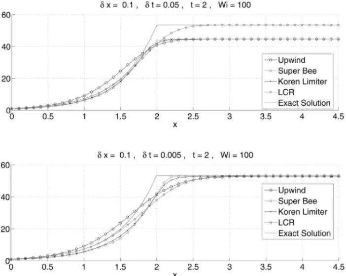
3.1 Influence ofδt
Takinga = 1,b = 2,W i =100,L = 4.5, δx = 0.1 and varyingδt, Figure 1 represents the perfil, att = 2, of the numerical solution of the equation (1.1) without LCR and with LCR. The solution provided by the LCR (2.10) always follows the growth of the exact solution. As expected the method with LCR suffers a dissipation at the contact discontinuity point of the solution; the same occurs with the other methods as well. Note that in cases without LCR the numerical solution only follows the adequate increasing of the exact solution asδtdecreases.
Figure 1: Behaviour of different methods for decreasingδt.
Table 1: Norm 2 relative error att=2 and absolute error at (t =2,x=4).
Relative Error att=2 (norm 2),W i=100
δt CFL LCR Upwind Superbee Koren 0.05 0.5 0.0611 0.1712 0.1623 0.1639 0.005 0.05 0.0933 0.0765 0.0772 0.0777
Absolute Error att =2,x =4 (W i=100)
δt CFL LCR Upwind Superbee Koren 0.05 0.5 0.0 8.8551 8.8551 8.8551 0.005 0.05 0.0 0.7838 0.7837 0.7837
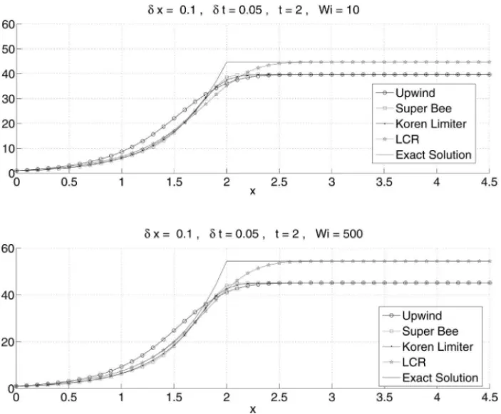
3.2 Influence ofWi
Takinga =1,b =2,L =4.5, δx =0.1 andδt =0.05, Table 2 presents the relative error, at
Figure 2: Behaviour of different methods for increasingW i.
Table 2: Norm 2 relative error att =2 and absolute error at (t =2,x=4).
Relative Error att=2 (norm 2),δt=0.05
W i LCR Upwind Superbee Koren
10 0.0585 0.1252 0.1109 0.1127 500 0.0613 0.1753 0.1666 0.1683
Absolute Error att=2,x=4 (δt=0.05)
W i LCR Upwind Superbee Koren
10 0.0 5.0492 5.0492 5.0492 500 0.0 9.2411 9.2411 9.2411
4 CONCLUSION
By using first order upwind in the convective term and explicit Euler in the transient term, we note that when including a source term in the advection equation it is also “inserted” a restriction of stability (2.6) to the spatial mesh that is influenced by the Weissenberg number. Thus, the higher
Also, corroborating with [3] and showing in a very concrete way, through a simple problem with exact solution, we can see that the numerical solution by methods without LCR does not follow the adequate growth of the analytical solution. This will certainly have consequences when a viscoelastic simulation is carried out. Asδt→0 there will be convergence and the higher order TVD schemes will approach the contact discontinuit better; upwind and LCR present strong dis-sipation near the contact discontinuity as expected. Numerical results verified these assumptions.
ACKNOWLEDGEMENTS
Thanks to FAPESP, for the financial support; Paper presented at CMAC – Sudeste in 2013.
RESUMO. O objetivo deste trabalho ´e estudar, por meio de uma equac¸˜ao simples, a afir-mac¸˜ao de que a instabilidade num´erica associada ao elevado n´umero Weissenberg em equa-c¸ ˜oes com termo fonte, pode ser resolvida pela utilizaequa-c¸˜ao da denominada representaequa-c¸˜ao por conformac¸˜ao logar´ıtmica. Vamos nos concentrar nas leis de conservac¸˜ao hiperb´olicas, mas mais especificamente na equac¸˜ao de advecc¸˜ao com termo fonte. O termo fonte imp˜oe a ne-cessidade de um equil´ıbrio el´astico, tanto quanto um equil´ıbrio convectivo (CFL), para a estabilidade. Ser´a visto que a representac¸˜ao de tal equac¸˜ao pela conformac¸˜ao logar´ıtmica remove a restric¸˜ao de estabilidade inerente para o equil´ıbrio el´astico apontado por Fattal & Kupferman [3] como causa do problema do alto n´umero de Weissenberg.
Palavras-chave:termo fonte, representac¸˜ao por conformac¸˜ao logar´ıtmica, problema do alto n´umero de Weissenberg.
REFERENCES
[1] A.M. Afonso, F.T. Pinho & M.A. Alves. The kernel-conformation constitutive laws. J. Non-Newtonian Fluid Mech.,167–168(2012), 30–37.
[2] J.A. Cuminato & M. Meneguette. Discretizac¸˜ao de equac¸˜oes diferenciais parciais: t´ecnicas de dife-renc¸as finitas. SBM, (2013).
[3] R. Fattal & R. Kupferman. Time-dependent simulation of viscoelastic flows at high Weissenberg number using the log-conformation representation. J. Non-Newtonian Fluid Mech., 126 (2005), 23–37.
[4] B. Koren. A robust upwind discretisation method for advection, diffusion and source terms, In: C.B. Vreugdenhil and B. Koren (Eds.), Numerical Methods for Advection-Diffusion Problems (pp. 117– 138). Vieweg, (1993).