Introducing the
q-Theil
index
M. Ausloos∗
GRAPES, ULG, B5a, Sart Tilman, B-4000 Liege, Euroland
J. Mi´skiewicz†
Institute of Theoretical Physics, Wrocaw University, pl. M. Borna 9, 50-204 Wrocaw, Poland (Received on 04 December, 2008)
Starting from the idea of Tsallis on non-extensive statistical mechanics and theq-entropynotion, we recall the Theil index T hand transform it into the T hq index. Both indices can be used to map onto themselves any time series in a non linear way. We develop an application of theT hqto the GDP evolution of 20 rich countries in the time interval [1950 - 2003] and search for a proof of globalization of their economies. First we calculate the distances between the “new” time series and to their mean, from which such data simple networks are constructed. We emphasize that it is useful to, and we do, take into account different time “parameters”: (i) the moving average time window for the raw time series to calculate theT hqindex; (ii) the moving average time window for calculating the time series distances; (iii) a correlation time lag. This allows us to deduce optimal conditions to measure the features of the network, i.e. the appearance in 1970 of a globalization process in the economy of such countries and the present beginning of deviations. Theqvalue hereby used is that which measures the overall data distribution and is equal to 1.8125.
Keywords: Econophysics, Time series analysis, Entropy
1. INTRODUCTION
Since the fundamental work of Boltzmann [1] the entropy concept has been developed and applied to a range of sub-jects going from elementary termodynamics and statistical mechanics through quantum physics e.g. [2], information theory [3] up to applications in biology e.g. [4–6] and econ-omy [7–9]. Recently Tsallis and many others in his path have shaken up the usual considerations on the entropy concept, in particular within Shannon information theory.
In fact, complex nonequilibrium systems can be often de-scribed by a superstatistics, which results from a superposi-tion of two statistics associated with two different time scales [7, 10–14]. The methods of extracting superstatistics param-eters from time series are discussed in [15]. In that line of thought, a special attention can be paid to the entropy of a time series.
On the other hand, the Theil [16] index is often used in economy and finance. It is defined through
T h(x;N) = 1 N
N
∑
i=tx
i hxii
ln xi
hxii
(1)
where the averagehxiis made over the ensemble of points N of the population of size N. It looks like the Shannon entropy but was invented to consider the event values them-selves, in particular the incomexi of agentiin a population ofNagents, rather than their probability of occurrence. One peculiarity is that it measures the individual’s share of income relative to the mean incomehxiiof the population. With ref-erence to information theory, Theil’s measure is a diffref-erence between its maximum entropy and its present entropy at that time. Thus from the Theil index one can look at correlations
∗Electronic address:[email protected] †Electronic address:[email protected]
between data sets, distances, hierarchies, and other usual fea-tures, through various techniques of data analysis, like those resulting after network constructions.
An interesting development is to consider that thexi quan-tity in Eq.(1) is time dependent. Thus one can generalize the Theil index in order to remap in a nonlinear way a time series x(t)into aT h(t), as done in Sect. 2 which recalls considera-tions outlined in [17]. Moreover in the spirit of non-extensive statistical entropy, following Tsallis considerations, it can be imagined to propose the q-Theilindex, as done in Sect. 2. The first application is here below made to macroeconomy time series, in particular to the GDP of the richest countries. Following up on studies of correlations between GDPs of rich countries [17–25], we have analyzed web-downloaded data on GDP, used as individual wealth signatures of a country’s economical state (“status”). We have calculated the fluctua-tions of the GDP and looked for correlafluctua-tions, and “distances”, as reported in Sect. 3.
Usually, a system is represented by a network, nodes being scalar agents, here the countries, while links are weights, i.e. here measures of distances between twoT h(t)representing GDP fluctuation correlations between two countries. In or-der to extract structures from the networks, we have averaged the time correlations in different windows. This allows more robustness in the subsequent network properties and reveals evolvingstatistical distances. In line with our previous works [17–20] we have examined three different network construc-tions. A discussion on economy globalization follows with a conclusion in Sect. 4. It is found that such a measure of col-lective habitsdoes fit the usual expectations defined by politi-cians or economists, i.e. common factors are to be searched for.
2. THEIL INDEX AND TSALLIS ENTROPY
time seriesA(t)into a new one through
T hA(t,T1) =
1
T1
t+T1
∑
i=t
Ai
hAi(t,T1) ln Ai
hAi(t,T1)
(2)
where the average hAi(t,T1) is made over the ensemble of points j in a time window of sizeT1, placed betweent and
t+T1:
hAi(t,T1)= 1
T1
t+T1
∑
j=tAj. (3)
Thus the Theil index is calculated for the interval[t,t+T1].
Applications of the Theil index notion can be found in other papers [17, 20], where the Theil index was applied to measure the economy globalization process.
In order to connect with Tsallis non extensive statistics we introduce theq-TheilindexT hAqfor a time seriesA(t)
T hAq(t,T1) =
1−∑t+T1
i=t (Ai/hAii(t,T1))
q
q−1 (4)
in the interval[t,t+T1]. Eq.(4) corresponds to Eq.(2) when
q→1.
In order to compare time series, their distance can be im-mediately introduced. Moreover the mean and standard devi-ations (std) of an ensemble of such distances can be used in further considerations. The distance between two time series (here the Theil-mapped time series) is hereby defined as the absolute value of the difference between mean values in the interval[t,t+T2]. Moreover the elements of the time series
can be taken at equal times or with the time lagτ, a possibility which we also take into consideration for generality purposes. Thus we define
dT hq(A,B)(t,T1,T2,τ)=|hT h
A
q(t,T1)−T hBq(t+τ,T1)i(t,T2)|. (5) In Eq.(5) the mean value denoted by brackets,h...i, is de-fined as in Eq.(3).
As a result we have three different time parameters:
1. theT1time window while calculating theT hqindex,
2. the time lagτ, and
3. the correlation windowT2.
Note: in the analysis both time windows (T hqand correla-tion) are used congruently so the total size of the time window is equal to the sum of theT hqand correlation time windows. Therefore the number of the generated networks is equal to the time series length minus the total time window size.
3. MACROECONOMY INDEX INPUT AND NETWORK
CONSTRUCTION
3.1. GDP data
GDP data sets of the richest OECD countries were used, i.e. Austria, Belgium, Canada, Denmark, Finland, France,
Greece, Ireland, Italy, Japan, the Netherlands, Norway, Por-tugal, Spain, Sweden, Switzerland, Turkey, U.K., U.S.A, and Germany, allowing for a linear superposition of the data be-fore the reunification in 1991 in the latter case; an All country is also invented as in previous works [17–20].1ThusN=21. The data starts in 1950 and finishes in 2003, so there are 54 data points in every time series.
3.2. Networks
The distance matrices obtained from Eq.(5) are analysed by constructing three network structures and analysing statis-tical properties of the distances between nodes. The follow-ing networks are considered: unidirectional minimal length path (UMLP), bidirectional minimal length path (BMLP) and locally minimal spanning tree (LMST). The algorithms gen-erating the mentioned networks are:
UMLP The network begins with an arbitrary chosen coun-try, – here the All councoun-try, then the closest neighbour-ing country is attached and becomes the end of the work. The next country closest to the end of the net-work is searched and attached. The process continues until all countries are attached to the network.
BMLP The network begins with the pair of countries with the smallest distance between them. Then the coun-try closest to the ends of the network are searched and those with shorter distance attached to the appropriate end. The algorithm is continued until all countries be-come nodes of the network.
LMST The root of the network is the pair of closest neigh-bouring countries. Then the country closest to any node is searched and attached. The algorithm is continued until all countries are attached to the network.
Notice that in the UMLP construction, All is at the begin-ing of the chain, while in the other two constructions, All is treated as a “normal” country. The BMLP and LMST net-work seeds are the appropriate pairs of the closest countries according to the appropriate distance matrix. The first two networks are linear, and essentially robust against a “pertur-bation”, as when removing or adding a country or in the case of a regrettable mathematical error, since they are based on a measure relative to a statistical mean, while the LMST is ob-vioulsy a tree, rather compact when only 21 data points, thus with very few branching levels, are involved in the construc-tion. It is known that such a tree is far from robust.
4. RESULTS
First let us report that aqvalue of the considered data set must be given. It could be let as a free parameter and one could find some optimal value according to some criterion,
1The set deviates somewhat from previous works [17, 19, 20] since there is
10 20 30 40 50 T2
0 10 20 30 40 50
T1
0 0.2 0.4 0.6 0.8 1 1.2
FIG. 1: Mean distance between countries deduced from T hq for
UMLP networks. The distance is averaged over the network links and the time. The values ofT1andT2are given on the vertical and horizontal axis respectively. Time lag value:τ=0 y. The color scale in use is indicated. A few numerical values are given in Table 5.
10 20 30 40 50
T2 0
10 20 30 40
T1
0 0.2 0.4 0.6 0.8 1 1.2 1.4 1.6 1.8 2
FIG. 2: Mean distance between countries deduced from T hq for
UMLP networks. The distance is averaged over the network links and the time. The size ofT1andT2are presented on the vertical and
horizontal axis respectively. Time lagτ=5 yrs. The color scale in use is indicated. A few numerical values are given in Table 5.
10 20 30 40
T2 0
10 20 30 40
T1
0 0.5 1 1.5 2 2.5 3
FIG. 3: Mean distance between countries deduced from T hq for
UMLP networks. The distance is averaged over the network links and the time. The size ofT1andT2are presented on the vertical and horizontal axis respectively. Time lagτ=10 yrs. The color scale in use is indicated. A few numerical values are given in Table 5.
10 20 30 40 50
T2 0
10 20 30 40 50
T1
0 0.1 0.2 0.3 0.4 0.5 0.6 0.7 0.8 0.9
FIG. 4: Mean distance between countries deduced from T hq for
BMLP networks. The distance is averaged over the network links and the time. The size ofT1andT2are presented on the vertical and horizontal axis respectively. Time lagτ=0 y. The color scale in use is indicated. A few numerical values are given in Table 5.
10 20 30 40 50
T2 0
10 20 30 40
T1
0 0.2 0.4 0.6 0.8 1 1.2 1.4 1.6 1.8 2 2.2
FIG. 5: Mean distance between countries deduced from T hq for
BMLP networks. The distance is averaged over the network links and the time. The size ofT1andT2are presented on the vertical and
horizontal axis respectively. Time lagτ=5 yrs. The color scale in use is indicated. A few numerical values are given in Table 5.
10 20 30 40
T2 0
10 20 30 40
T1
0 0.5 1 1.5 2 2.5 3
FIG. 6: Mean distance between countries deduced from T hq for
10 20 30 40 50 T2
0 10 20 30 40 50
T1
0 0.1 0.2 0.3 0.4 0.5 0.6 0.7 0.8 0.9
FIG. 7: Mean distance between countries deduced from T hq for
LMST networks. The distance is averaged over the network links and the time. The size ofT1andT2are presented on the vertical and horizontal axis respectively. Time lagτ=0 y. The color scale in use is indicated. A few numerical values are given in Table 5.
10 20 30 40 50
T2 0
10 20 30 40
T1
0 0.2 0.4 0.6 0.8 1 1.2 1.4 1.6 1.8 2
FIG. 8: Mean distance between countries deduced from T hq for
LMST network. The distance is averaged over the network links and the time. The size ofT1andT2are presented on the vertical and
horizontal axis respectively. Time lagτ=5 yrs. The color scale in use is indicated. A few numerical values are given in Table 5.
10 20 30 40
T2 0
10 20 30 40
T1
0 0.5 1 1.5 2 2.5 3 3.5
FIG. 9: Mean distance between countries deduced from T hq for
LMST networks. The distance is averaged over the network links and the time. The size ofT1andT2are presented on the vertical and horizontal axis respectively. Time lagτ=0 yrs. The color scale in use is indicated. A few numerical values are given in Table 5.
or a few criteria. Here below, i.e. for the GDP time series in 1950-2003 for the countries defined in Sec.3.1 we have calcu-lated theqvalue for the following considerations by the max-imum likelihood estimator [26], as for Tsallis entropy, and foundq=1.8315, hereby used to calculate distances through Eq.(4) and Eq.(5). It is fair to recall that Borges in [27] cal-culated the (Tsallis entropy)qvalue for GDP of USA, Brasil, Germany and UK. He found aqvalue varying from 1.4 (UK) up to 2.1 (Brasil), and for USA,q=1.7.
4.1. q-Theildistance statistics
In our analysis UMLP, BMLP and LMST networks were constructed for all time windows ranging from T1=5 yrs,
T2=1 y moving along the time axis by a one year step.
Eleven time lag values were considered: τ∈[0,1, . . . ,10]. TheT1,T2andτparameters satisfy the inequalityT2+T3+
τ≤54 yrs, so the number of generated networks (Net) de-pends on the time window sizes and is equal toNNet =54−
T1−T2−τ, for a given triplet, - times 3, due to the type of
net-work considered. In total this is a huge number of netnet-works. Therefore some cases are to be extracted for the present re-port.2 Different presentations can be made, in a three dimen-sional time coordinate space. We propose a vizualisation of the data through a spectrogram method, using for thexand
yaxis the time windowT2andT1respectively for a givenτ.
The data values are represented by a colored pixel in a con-venient order.3 The results of calculations of the mean but also values of the corresponding standard deviations are here below presented.
The mean value and standard deviation of the distances be-tween nodes as a function of theT1 andT2are presented in
Figs. 1 - 9 for the time lagτ=0,5,10 yrs. The largest value of the mean distance, the minimum mean distance, the max-imum and minmax-imum standard deviations as a function of the time windowsT1,T2and time lags are presented in Table 5.
It can be first generally observed that the mean distance be-tween countries and the corresponding standard deviation are the biggest for UMLP networks and the smallest for LMST networks. It is also worth noticing that the mean distance de-pends on the time lag value. If the time lag is large the mean distance is large as well. The maximum of the mean distance occurs for the longestT1and the shortestT2windows sizes.
The minimum mean distance is found with the oposite com-bination of the time windows sizes, i.e. smallT1and largeT2.
The standard deviations increase with the time lag and are the largest ones in the case of the longest considered time lag.
2All cases are available from the authors upon request.
3The results are presented in grey tones, but online figures are available in
0 0.002 0.004 0.006 0.008 0.01 0.012 0.014 0.016 0.018 0.02
1965 1975 1985 1995 1950 1960 1970 1980
mean
T1=5 yrs, T2 = 10 yrs
tau=0 yrs tau = 2 yrs tau=4 yrs
tau=6 yrs tau=8 yrs tau=10 yrs
FIG. 10: Yearly evolution of the mean and standard deviation of the links between nodes for the UMLP network deduced fromT hq
analysis of GDP countries, whenT1=5 yrs,T2=10 yrs for different
time lagsτ.
0 0.02 0.04 0.06 0.08 0.1 0.12 0.14 0.16
1965 1975 1985 1995 1950 1960 1970 1980
mean
T1=10 yrs, T2 = 5 yrs
tau=0 yrs tau = 2 yrs tau=4 yrs
tau=6 yrs tau=8 yrs tau=10 yrs
FIG. 11: Yearly evolution of the mean and standard deviation of the links between nodes for the UMLP network deduced fromT hq
analysis of GDP countries, whenT1=10 yrs,T2=5 yrs for different
time lagsτ.
4.2. q-Theilnetwork evolution
For further discussion the following time window sizes were chosen, i.e. (T1=5 yrs, T2=10 yrs),(T1=10 yrs,
T2=5 yrs),(T1=10 yrs,T2=10 yrs),(T1=15 yrs,T2=15
yrs), for the three time lagsτ=0,5,10 yrs. The evolutions of mean distance between countries and the corresponding standard deviations for these chosen time windows sizes are
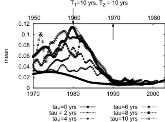
0 0.02 0.04 0.06 0.08 0.1 0.12 0.14 0.16
1970 1980 1990 2000 1950 1960 1970 1980
mean
T1=10 yrs, T2 = 10 yrs
tau=0 yrs tau = 2 yrs tau=4 yrs
tau=6 yrs tau=8 yrs tau=10 yrs
FIG. 12: Yearly evolution of the mean and standard deviation of the links between nodes for the UMLP network deduced fromT hq
anal-ysis of GDP countries, whenT1=10 yrs,T2=10 yrs for different time lagsτ.
0 0.05 0.1 0.15 0.2 0.25 0.3 0.35
1980 1990 2000 1950 1960 1970
mean
T1=15 yrs, T2 = 15 yrs
tau=0 yrs tau = 2 yrs tau=4 yrs
tau=6 yrs tau=8 yrs tau=10 yrs
FIG. 13: Yearly evolution of the mean and standard deviation of the links between nodes for the UMLP network deduced fromT hq
anal-ysis of GDP countries, whenT1=15 yrs,T2=15 yrs for different
time lagsτ.
0 0.002 0.004 0.006 0.008 0.01 0.012 0.014 0.016 0.018
1965 1975 1985 1995 1950 1960 1970 1980
mean
T1=5 yrs, T2 = 10 yrs
tau=0 yrs tau = 2 yrs tau=4 yrs
tau=6 yrs tau=8 yrs tau=10 yrs
FIG. 14: Yearly evolution of the mean and standard deviation of the links between nodes for the BMLP network deduced fromT hq
analysis of GDP countries, whenT1=5 yrs,T2=10 yrs for different
time lagsτ.
presented in Figs. 10-21. Arrows and straight lines indicate remarkable features.
The general observations to be made at this stage are the following
• In all considered networks (UMLP, BMLP and LMST) and for all window sizes three types of evolution can be distinguished: increase, decrease and relatively stable mean distance between countries.
-0.02 0 0.02 0.04 0.06 0.08 0.1 0.12 0.14 0.16 0.18
1965 1975 1985 1995 1950 1960 1970 1980
mean
T1=10 yrs, T2 = 5 yrs
tau=0 yrs tau = 2 yrs tau=4 yrs
tau=6 yrs tau=8 yrs tau=10 yrs
FIG. 15: Yearly evolution of the mean and standard deviation of the links between nodes for the BMLP network deduced fromT hq
-0.02 0 0.02 0.04 0.06 0.08 0.1 0.12
1970 1980 1990 2000 1950 1960 1970 1980
mean
T1=10 yrs, T2 = 10 yrs
tau=0 yrs tau = 2 yrs tau=4 yrs
tau=6 yrs tau=8 yrs tau=10 yrs
FIG. 16: Yearly evolution of the mean and standard deviation of the links between nodes for the BMLP network deduced fromT hq
anal-ysis of GDP countries, whenT1=10 yrs,T2=10 yrs for different
time lagsτ.
0 0.05 0.1 0.15 0.2 0.25 0.3 0.35
1980 1990 2000 1950 1960 1970
mean
T1=15 yrs, T2 = 15 yrs
tau=0 yrs tau = 2 yrs tau=4 yrs
tau=6 yrs tau=8 yrs tau=10 yrs
FIG. 17: Yearly evolution of the mean and standard deviation of the links between nodes for the BMLP network deduced fromT hq
anal-ysis of GDP countries, whenT1=15 yrs,T2=15 yrs for different time lagsτ.
• These three types of evolution are better seen for long lag time (τ>5 yrs). Therefore the lag time seems to be crucial in any analysis and discussion of the global-ization process. This might suggest that some countries play a role of leaders while other follow their way.
• It is worth noticing that for the very long lag timeτ= 10 yrs and time windows [(T1=5 yrs,T2=10 yrs),
(T1=10 yrs,T2=5yrs),(T1=10yrs,T2=10yrs)] the
0 0.002 0.004 0.006 0.008 0.01 0.012 0.014 0.016 0.018 0.02
1965 1975 1985 1995 1950 1960 1970 1980
mean
T1=5 yrs, T2 = 10 yrs
tau=0 yrs tau = 2 yrs tau=4 yrs
tau=6 yrs tau=8 yrs tau=10 yrs
FIG. 18: Yearly evolution of the mean and standard deviation of the links between nodes for the LMST network deduced fromT hq
analysis of GDP countries, whenT1=5 yrs,T2=10 yrs for different time lagsτ.
0 0.02 0.04 0.06 0.08 0.1 0.12 0.14 0.16 0.18 0.2
1965 1975 1985 1995 1950 1960 1970 1980
mean
T1=10 yrs, T2 = 5 yrs
tau=0 yrs tau = 2 yrs tau=4 yrs
tau=6 yrs tau=8 yrs tau=10 yrs
FIG. 19: Yearly evolution of the mean and standard deviation of the links between nodes for the LMST network deduced fromT hq
analysis of GDP countries, whenT1=10 yrs,T2=5 yrs for different
time lagsτ.
0 0.02 0.04 0.06 0.08 0.1 0.12
1970 1980 1990 2000 1950 1960 1970 1980
mean
T1=10 yrs, T2 = 10 yrs
tau=0 yrs tau = 2 yrs tau=4 yrs
tau=6 yrs tau=8 yrs tau=10 yrs
FIG. 20: Yearly evolution of the mean and standard deviation of the links between nodes for the LMST network deduced fromT hq
anal-ysis of GDP countries, whenT1=10 yrs,T2=10 yrs for different time lagsτ.
maximum of the mean distance occurs around 1960,
• since then the size of the network(s) is fast decreasing over a decade up to 1970 and
• thereafter remains small and relatively stable up to 2000 or so
• when the mean size seems to reincrease.
0 0.05 0.1 0.15 0.2 0.25 0.3 0.35
1980 1990 2000 1950 1960 1970
mean
T1=15 yrs, T2 = 15 yrs
tau=0 yrs tau = 2 yrs tau=4 yrs
tau=6 yrs tau=8 yrs tau=10 yrs
FIG. 21: Yearly evolution of the mean and standard deviation of the links between nodes for the LMST network deduced fromT hq
5. CONCLUSIONS
In conclusion, the most interesting results of this analysis are
• The analysis shows the existence of a globalization pro-cess starting from 1960 till 1970 and its stabilisation thereafter, followed by a destabilisation after 2000 as observed in the decrease of the network size.
• The observation of the globalization process does not depend on the type of network constructed.
• The mean distance between countries and the corre-sponding std are the largest for the UMLP networks and the smallest for the corresponding LMST networks.
• With increasing time lag the Theil mapping window
sizeT1 at which the maximum of the network size is
found is always decreasing.
• The globalization process is better seen if the lag time is greater than 5 yrs, - which might be considered as the time needed for some synchronization process, but is also in fact commensurate with most government life times and election time intervals. These conjectures suggest further investigations.
• Even though for large time lags the mean values are large, the globalization evolution is the same as for short time lags (greater than 5 yrs); thus a large time lag magnifies the globalization process feature which is, therefore, easier to observe.
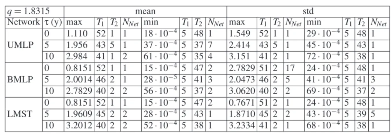
q=1.8315 mean std
Network τ(y) max T1 T2 NNet min T1 T2 NNet max T1 T2 NNet min T1 T2 NNet
0 1.110 52 1 1 18·10−4 5 48 1 1.549 52 1 1 29·10−4 5 48 1 UMLP 5 1.956 43 5 1 37·10−4 5 37 7 2.414 43 5 1 45·10−4 5 43 1 10 2.984 41 1 2 61·10−4 5 35 4 3.151 41 2 1 72·10−4 5 38 1 0 0.8151 52 1 1 15·10−4 5 47 2 2.7829 51 2 17 24·10−4 5 48 1
BMLP 5 2.0014 46 2 1 28·10−5 5 41 3 2.0473 46 2 5 41·10−4 5 41 3 10 2.7829 40 2 2 56·10−4 5 37 2 3.0620 40 2 2 69·10−4 5 37 2 0 0.8151 52 1 1 15·10−4 5 47 2 0.7671 51 2 1 24·10−4 5 48 1 LMST 5 1.9609 45 2 2 28·10−4 5 43 1 1.8710 45 2 2 43·10−4 5 39 5 10 3.2012 40 2 2 52·10−4 5 38 1 3.2334 41 2 1 68·10−4 5 38 1
TABLE I: The maximum mean distance, the minimum mean distance, the maximum and minimum standard deviations resulting for each type of network, for a few characteristicsτvalues are given whenT hqis calculated forq=1.8315. Recall that the “mean” is that of the distances between nodes on the indicated network in the ensemble of networks generated for the given time windows. The values of the averaging windowsT1andT2when this maximum (minimum) occurs are indicated; the corresponding number of networks (NNet) used for the statistics is also indicated.
Of course much more work is in order to connect the above to some non extensive thermostatistics ideas. To search for a robust (“optimal”)qvalue and the significance of theq-Theil
index are open questions. Finally let us stress the interest of studying graphs, in particular to derive weighted networks such as in this paper, in order to have some comparative data organisation coherence.
The ordinaryq=1 case has been presented and discussed at the 2009 Medyfinol congress [28], where several figures illustrate the development. In short, there is neither much dif-ference between the numerical results forq=1 or not, nor the main macroeconomic conclusions. However we have found that theq=1 development leads to less “stability” or “co-herence” in the results, in particular when they are observed
as a function of the time window. Such visual features can-not be simply quantified through statistical tests. Therefore we let the readers compare for him/herself the data in both publications.
5.1. Acknowldgements
Thanks to the organizers of NEXT2008 in Foz do Iguacu, Parana, in particular Luis C. Malacarne and Reino S. Mendes, plus kind thanks to Thais Pedreira for their welcome and care-ful attention to MA needs at the meeting. Let C. Tsallis be congratulated for his great insight, what he brought to mod-ern equilibrium thermostatistics and for suggesting MA par-ticipation at such a meeting.
[1] L. Boltzmann, Vorlesungen ber Gastheorie: 2 Volumes (Leipzig, 1895/98).
[2] S. Gheorghiu-Svirschevski, Phys. Rev. A 63, 022105 (2001).
[3] C. E. Shannon, Bell Syst. Tech. J. 30, 50 (1950).
[4] J. L. Ruiz de la Torre, A. Velarde, and X. Manteca, Anim. Be-hav. 59, 269 (2000).
[5] D. R. Brooks and E. O.Wiley, Evolution As Entropy: Toward a Unified Theory of Biology (University of Chicago Press, 1988).
[6] C. T. Murray Gell-Mann, Nonextensive Entropy: Interdisci-plinary Applications (Oxford University Press, 2004).
[8] J. A. Duro and J. Esteban, Econom. Lett. 60, 269 (1998).
[9] J. A. James and M. Thomas, J. Income Distrib. 9, 39 (2000).
[10] C. Beck and E. G. D. Cohen, Physica A 322, 267 (2003).
[11] A. Mathai and H. Haubold, Physica A 385, 493 (2007).
[12] H. Touchette and C. Beck, Phys. Rev. E 71, 016131 (2005).
[13] C. Tsallis and A. M. C. Souza, Phys. Rev. E 67, 026106 (2003).
[14] J.-P. Bouchaud and M. Potters, Theory of Financial Risk and Derivative Pricing (Cambridge University Press, 2003).
[15] C. Beck, E. G. D. Cohen, and H. L. Swinney, Phys. Rev. E 72, 056133 (2005).
[16] H. Theil was a Dutch econometrician who was born on13 Oc-tober 1924 in Amsterdam, graduated from the University of Amsterdam, succeeded to Jan Tinbergen at the Erasmus Uni-versity Rotterdam, moved and taught later in Chicago and at the University of Florida. He died in 2000.
[17] J. Miskiewicz, Physica A 387, 6595 (2008).
[18] J. Miskiewicz and M. Ausloos, Acta Phys. Pol. B 36, 2477 (2005).
[19] J. Miskiewicz and M. Ausloos, Int. J. Mod. Phys. C 17, 317 (2006).
[20] J. Miskiewicz and M. Ausloos, Physica A 387, 6584 (2008).
[21] M. Ausloos and R. Lambiotte, Physica A 382, 16 (2007).
[22] M. Ausloos and M. Gligor, Eur. Phys. J. B 57, 139 (2007).
[23] M. Gligor and M. Ausloos, J. Econ. Integration 23, 297 (2008).
[24] M. Ausloos and M. Gligor, Physica A 114, 491 (2008).
[25] M. Gligor and M. Ausloos, Eur. Phys. J. B 63, 533 (2008).
[26] A. C. C. Shalizi and M. Newman, Power-law distributions in empirical data, E-print, arXiv:0706.1062 (2007).
[27] E. P. Borges, Physica A 334, 255 (2004).