Braz. J. Phys. vol.37 número2B

(1)

626 Brazilian Journal of Physics, vol. 37, no. 2B, June, 2007

Effects of Solar Neutrinos Scale on Atmospheric Neutrino Flux

D. R. Grating and O. L. G. Peres

Universidade Estadual de Campinas, Instituto de F´ısica Gleb Wataghin, Departamento de Raios C´osmicos, C.P. 6165, Campinas, 13083-970, SP, Brazil

Received on 13 December, 2006

In this work we try to understand the phenomena of neutrino oscillations, and use this to obtain a more pre-cise description of the atmospheric neutrino data. The two neutrino oscillation mechanism solves the problem of the up-down muon neutrino asymmetry successfully. Our main motivation is to describe the excess of events of electron-neutrino type found in the SuperKamiokande results at low energies when compared with the pre-dictions of the two-generation neutrino oscillation. To do this we generalize the oscillation model from two to three neutrino flavors, opening the possibility of oscillation between electron neutrino type and the others. Then we obtain a semi-analytic solution of the three flavors problem using the neutrino phenomenological limits on oscillation parameters, squared masses differences and mixing angles. For this we must take into account matter effects on the electronic neutrino when it cross the Earth and has its oscillation pattern changed.

Keywords: Neutrino oscillations; Atmospheric neutrinos

I. INTRODUCTION

Atmospheric neutrinos have their origin in the cosmic ray collisions with Earth’s atmosphere. In this process are formed initially hadrons whose decay mainly into pions and kaons that have neutrinos as product of it’s decay. As kaons are pro-duced in more energetic and rare showers, the principal decay mode for neutrino production is π→ µ + νµ followed by µ_→e + νe+ν¯µ, that implies that the ratio between muon-type and electron-muon-type neutrino fluxes is equal two. As shown in Fig .(1), the atmospheric neutrino problem is related to the fact the SuperKamiokande (SK)[1] results of measurement of muon events induced by atmospheric neutrinos, is smaller than the theoretical previsions [2, 3]. This deficit in muon-like neutrino events depends on the neutrino zenith angle and may be even 50% whencosθz→ −1. The fact that this deficit depends on the zenith angle, θz, excludes the possibility to describe by a renormalization in the SK data. To explain this phenomena is used the flavor oscillation model in two gen-erations of neutrinos induced by mass, whose describes the experimental data.

II. NEUTRINO FLAVOR OSCILLATIONS

A. Vacuum oscillation in two generations

This is the most simple case of the flavor oscillation model [4], which assumes that the flavor neutrino eigenstates,

|ναi, are not the eigenstates of Hamiltonian, but a linear

atmospheric neutrino case, and can be written as

|ναi=

3

∑

i=2

U_α∗_i_|νii, (1) whereU is the neutrino mixing matrix [5, 6], for two neu-trino generations. Explicitly, the Eq .(1) may be written as a

function of the atmospheric mixing angleθatm=θ23as,

µ

νµ

ντ

¶ =

µ

cosθ23 senθ23

−senθ23 cosθ23 ¶ µ

ν2 ν3

¶

. (2)

So, the temporal evolution of flavor neutrinos must be given by the evolution of the mass eigenstates,

id dt

µ

νµ

ντ

¶

=U HU† µ

νµ

ντ

¶

, (3)

whereH=diag(E2,E3), andEiis the eigenvalue of the|νii. As a direct consequence of this, the probability of for a given a initial flavor neutrino eigenstate|νµito change to the|ντi

neutrino flavor state, it is not zero but:

P(νµ→ντ) =sen2(2θ23)sen2 µ

∆m2₃₂L 2E

¶

, (4)

where∆m2_atm=∆m₃₂2 _≡m2₃₋m2₂is atmospheric squared mass difference. We also have the solar squared mas difference de-fined as∆m2_⊙=∆m₂₁2 _≡m2₂₋m2₁.

This is not zero if the mass eigenvalues are different of zero and not all degenerated, because if∆m2₃₂=0 there is no oscil-lation. Eq .(4) generates the solid lines in Fig .(1)that are in agreement with the muon-like neutrino data from SK.

B. Why to generalize to three generations?

As pointed by [7], a inspection of the first column in Fig. (1) with respect to electron-like neutrino events, a ex-cess of events in the SK data at low energies (P<400 GeV) when compared to predictions with the two neutrino oscil-lations taken account [9]. So we generalize the oscillation model to three neutrino generations and allow the possibility of oscillation between the electron neutrino and the others.

(2)

D. R. Grating and O. L. G. Peres 627

FIG. 1: SuperKamiokande results [8] for the zenith dependence of the atmospheric data (points) compared with the theoretical simula-tions (little boxes) from Hondaet. al[2]. The prediction with oscilla-tion is denoted by a solid line. From top to bottom, respectively three charged lepton momentum bins, as can be seen in the plots. From left to right, we have the different samples: electron-like, muon-like and muon-like multi-ring events

FIG. 2: In the picture are shown the density filled byνeas a function of distance L. In the legend, from the top to bottom we haveθz= 180o→100o.

lepton to interact by weak charged current (CC), in which the mediator boson is massive and electrically charged,W±. This interaction gives rise to a effective potential due to electrons in a medium. For the Earth’s interior a simple calculation [10] gives

Ve=

√

2GFNe∼3.10−14 µ _ρ

10g/cm3 ¶

eV, (5)

FIG. 3: Oscillation probabilities as a function of the distance L for different values ofδparameter in units of(10−11₎_eV.

whereGF is the Fermi constant, Ne is the number of elec-trons in the medium, andρe is the electronic number den-sity [11, 12]. In Fig. (2) we showρeas a function of the dis-tance traveled in Earth,L=−2Rcosθz, whereRis the Earth’s radius, for different values of the zenith angleθz.

As shown in ref. [10], for anti-neutrinos the signal ofVCC is opposite for the signal to neutrinos. The changes on oscilla-tions patterns depend on the local electronic density in Earth’s interior. We called it as medium effect.

C. How to generalize to three neutrino generations ?

In the presence of a medium, the effective Hamiltonian may be written as,

H=

µ U M2U†

2E +V ¶

, (6)

where the mass matrix M2 is M2 =

diag¡0,∆m2₂₁,∆m₃₁2 ¢ , and V = (Ve,0,0) . So in three neutrino generations and taking into account the medium effects, the evolutions of|ναiis given by,

id dt|ναi=

Ã

U23U13U12M2U12†U † 13U

† 23

2E +V

!

|ναi, (7)

where|ναiis a combination of three mass eigenstates,

|ναi=

3

∑

i=1

U_α∗_i_|νii. (8)

(3)

628 Brazilian Journal of Physics, vol. 37, no. 2B, June, 2007

∆m2₂₁=∆m2_⊙=8 10−5eV2[1, 13], and∆m2₃₂=∆m2_{AT M}= 2.5 10−5eV 2 [9, 14] so in our calculations we use the ap-proximation ∆m2

⊙<<∆m2atm. For mixing angles we have tan2₍_θ

⊙) = 0.4, sen2(θatm) = 1/2, and sen2(θ13)< 0.1. Thereforeθ13is a small angle and the others two are large.

Now we apply two rotations in the eigenstate base to trans-form the 3×3 system in other two, one 2×2 and a second 1×1. The first rotation is|ναi=U23U13|ν′αi. In the basis

|ν′

αi,

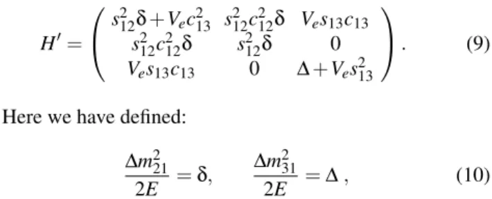
H′=  

s2₁₂δ+Vec213 s212c212δ Ves13c13 s2₁₂c2₁₂δ s2₁₂δ 0 Ves13c13 0 ∆+Ves213



. (9)

Here we have defined:

∆m2₂₁ 2E =δ,

∆m2₃₁

2E =∆, (10)

whereδand∆are the inverse of the oscillation lengths of solar and atmospheric neutrinos.

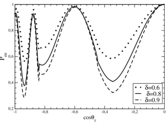
FIG. 4: Oscillation probabilities as a function ofcosθZfor different values ofδparameter in units of(10−11₎_eV.

The second rotation is_|ν′

αi=U13′ |ν′′αi, where the the

rota-tion angleθ′₁₃is such that,

s′₁₃= s13c132EVe 2EVes213+∆m231

∼ 2θ13EVe ∆m2

31+2EVeθ213

, (11)

thenθ′_{is a small angle also.}

In the propagation basis the Hamiltonian have the approxi-mated form, because the hierarchies of solar and atmospheric scale and smallness ofθ13.

H′′_∼  

s2₁₂δ+Vec213 s12c12δ ∼0 s12c12δ c212δ ∼0

0 0 ∆+Ves213 

, (12)

that implies in the decoupling of the tau neutrino state in the rotate basis,ν′′

τ. So by these two rotations we may write the

2×2 sub-system as,

id dt

µ

νe′′

νµ′′ ¶

= µ

s2₁₂δ+Vec213 s12c12δ s12c12δ c212δ

¶ µ

νe′′

νµ′′ ¶

(13)

and the sub-system 1×1

id dtν

′′

τ= (s′13s13c13Ve+∆+Ves213)ν′′τ (14)

Physically speaking, the two oscillation scales represent different orders of magnitude, i.e. the atmospheric one os-cillates faster than the solar one. When the oscillation due atmospheric scale is influencing the system the solar scale still not manifest. When the solar scale turns relevant the at-mospheric mechanism had oscillated so many times that the best we can observe is a average value.

In the propagation basis the S′′ matrix of amplitudes of probabilities have the form,

¯ S′′=

 

A′′_eeeiφ1 _A′′

µeeiφ2 0 A′′_µeeiφ2 _A′′

µµeiφ4 0 0 0 A′′_ττeiφ3



. (15)

where we obtain the coefficientsA′′_αβby numerical evaluation of Eq .(13), and the probabilities are given asP_α′′_→_β=|A′′_αβ_|2, andφiare oscillation phases, i=1,2,3.

III. PRELIMINARY RESULTS

We defineP2≡Pνe→νµ =|A′′eµ|2 as the probability of fla-vor transition in the propagation basis. The Fig. (3) show P2 as a function of the distance L traveled in the Earth for cos(θz) = −1.0, that means, for neutrinos that cross the entire Earth. We show the changes in the oscillation pattern when neutrinos cross regions with have different densities. In the Fig. (4) we showP2for the same values ofδbut as a function of the zenith angle (cosθz). For values ofcosθz<−0.85 neu-trino crosses the Earth’s core and in this region all the curves are in phase, that means that the oscillation length in this re-gion is not dependent of theδparameter.

A. Results in flavor basis

In the flavor basis the S matrix has the form,

S=U23U13U13′ +13′S′′U₁₃†₊₁₃′U23† , (16) and we will define the probabilities asP(να→νβ) =Pα→β,

(4)

D. R. Grating and O. L. G. Peres 629

FIG. 5: Probability of electronic neutrino survival as a function of cosθzfor different values ofδin units of(10−11)eV.

Pe_→e = 1−P2(c′′13)4−2(c′′13)2(s′′13)2 ³

1−p

1−P2cosφ23 ´

Pe→µ = (c′′13)2(s′′13)2s223 ³

1₋2p1₋P2cosφ23+ (1−P2) ´

+ 2(c′′13)2s′′13s23c23 ³p

P2cosφ13− p

(1−P2)P2cosφ12 ´

+ (c′′₁₃)2c2₂₃P2

Pe_→τ = (c′′13)2(s′′13)2c223 ³

1−2p1−P2cosφ23+ (1−P2) ´

+ 2(c′′₁₃)2_s′′ 13s23c23

³p

(1−P2)P2cosφ12− p

P2cosφ13 ´

+ (c′′13)2s223P2, (17)

whereφi j=φi−φj.

We plot in Fig. (5) the probability of survival of electronic neutrino given by Eq .(17) as a function ofcosθz. Again we note that forcosθz<−0.85 the phase of oscillation patterns is enhanced due to interaction with the electrons in the medium.

IV. CONCLUSIONS

This paper contains the our primary results that are summa-rized below.

Upon generalizing of the neutrino flavor oscillation model from two to three neutrino flavors, we verify also oscillations betweenνe→νµ which depends on ∆m221 andθ12 that are parametrized by by solar neutrino scale. This oscillations also dependents ofθ13, and have their pattern changed due to in-teraction ofνewith the electrons in the medium, when theνe realizes transitions between zones with densities in the Earth’s interior.

We conclude remembering that this medium effects plays an important rule in evolution ofνein the Earth’s interior, as shown in Figs .(3, 4, 5). Since for low energies initially there are approximately two times more muon neutrinos that elec-tron neutrinos, the medium effects would enhance the oscil-lation and causes the excess of electron neutrino in Sub-GeV region forcosθz→ −1 that was referred above in this work. From Eqs .(17) we see a dependence of the medium effects with respect to θ23 andθ13, such that this medium effects would be used to determinate the octant ofθ23 and impose limits onθ13, as pointed by [7].

[1] The SuperKamiokande Collaboration, S. Fukudaet al., Phys. Rev. Lett.81, 1158 (1999);ibid,85, 3999 (2000).

[2] M. Honda, T. Kajita, arXiv:astro-ph/0404457.

[3] T. K. Gaisser and M. Honda, Ann. Rev. Nucl. Part. Sci.52, 153 (2002)

[4] B. Pontecorvo, J. Exptl. Theoret. Phys.33, 549 (1957);ibid.34, 247 (1958).

[5] Z. Maki, M. Nakagawa, and S. Sakata, Prog. Theor. Phys.28, 870 (1962).

[6] Particle Data Group, S. Eidelmanet al., Phys. Lett. B592, 1 (2004).

[7] O. L. G. Peres, A. Yu. Smirnov, Nucl. Phys. B680, 479 (2004), and references cited there.

[8] SuperKamiokande Collaboration, Y. Ashieet al., Phys. Rev. D

71, 112005, (2005).

[9] The Super-Kamiokande Collaboration, S.Fukuda et al., arXiv:hep-ex060411.

[10] C. W. Kim, A. Pevsner.Neutrinos in Physics and Astrophysics, Hardwood, (1995).

[11] A.M. Dziewonski, D.L. Anderson, Physics of the Earth and Planetary Interiors,25, 297 (1981).

[12] E. Lisi, D. Montanino, Phys. Rev. D56, 1792 (1997).

[13] SNO Collaboration, B. Aharmim et al., Phys. Rev. C 72, 055502 (2005).