The Effect of Correlated Noise in a Gompertz Tumor Growth Model
Anita Behera School of Biomedical Sciences,
Queen’s University of Belfast, BT9 7AB, United Kingdom
S. Francesca C. O’Rourke School of Mathematics & Physics
Queen’s University of Belfast, BT7 1NN, United Kingdom
Received on 3 April, 2008
We study the effect of noise in an avascular tumor growth model. The growth mechanism we consider is the Gompertz model. The steady state probability distributions and average population of tumor cells are analyzed within the Fokker-Planck formalism to investigate the importance of additive and multiplicative noise. We consider the effect of correlation on tumor growth for both the case of nonzero and zero correlation time. It is observed that the Gompertz model, driven by correlated noise exhibits a stochastic resonance and phase transition. This behaviour is attributed to multiplicative noise. In the case of nonzero correlation time, it is found that the correlation strength and correlation time have opposite effects on the steady state probability distribution. The Gompertz model simulations are also shown to be in qualitative agreement with another similiar non-bistable system, the logistic model.
Keywords: Fluctuation phenomena; Random processes; Noise; Brownian motion
I. INTRODUCTION
Much of the attention in the recent years has been directed towards nonlinear physics and its application to uncover bio-logical complexities. Studies have confirmed the role of noise in the nonlinear stochastic systems [1]. In recent years the Fokker-Planck equation has become one of the important ap-proaches in the studies of nonlinear dynamics based on sto-chastic form [2, 3].
Tumor growth is a complex process. It has been a chal-lenge for many years to search for a suitable growth law of tu-mors. Mathematical models based on mathematical equations such as the Gompertzian, logistic and exponential equations are used as a basic tool for describing avascular tumor growth [4–6]. It has been realized that tumor growth is governed by environmental fluctuations [7]. It has also been shown that quite often there are discrepancies between theoretical predic-tions and clinical data due to more or less intense environ-mental fluctuations [8]. Ferreiraet al[6] analyzed the effect of distinct chemotheraputic strategies for the growth of avas-cular tumors. This study confirmed that an environment like chemotherapy affects tumor growth behaviour and may lead to morphological transitions under certain conditions.
Stochastic modelling using the Fokker-Planck equation has been recently applied to the logistic equation to study the steady state properties of avascular tumor growth driven by Gaussian correlated additive and multiplicative white noise by [9]. This work has been extended to consider the nonzero correlation time between additive and multiplicative noise by [10]. However among avascular tumor growth power laws the Gompertz model has been the most broadly and successfully applied to fit the experimental data [11–13]. Other successful applications in the literature of the Gompertz equation to can-cer cell growth include [14–16]. These models are however deterministic models. In this article we wish to consider the
Gompertz model from a stochastic viewpoint by examining the steady state properties of Gompertzian tumor cell growth driven by correlated noise. The Gompertz model has not been analyzed in the literature before in this context. In addition we extend our study to consider the nonzero correlation time for the Gompertz model.
The plan of this paper is as follows. Calculational details outlining the theoretical formulation of the Fokker-Planck equation applied to avascular tumor growth laws are presented in Sec.II. Sec.III presents the results for the steady state prop-erties and average cell populations of the Gompertz model driven by cross-correlated additive and multiplicative noise for the case of zero correlation time between noises. In Sec.IV we consider nonzero correlation time and present the results for the steady state properties of the Gompertz model driven by cross-correlated noise for the case of nonzero correlation time. We use our model to simulate the behaviour of the lo-gistic model of [9], [19], and [10] and compare with the results obtained from the Gompertz model.
Finally in Sec.V we discuss our conclusions.
II. THEORETICAL FORMULATION BASED ON THE FOKKER-PLANCK EQUATION
Avascular tumor growth laws may be described by a single deterministic differential equation,
dx
dt =f(x) withx(0) =x0, (1) where f(x)describes the tumor cell growth dynamics andx0 is the initial tumor size.
growth factors or host vasculature,(iv)tumor volume is pro-portional tox(t), the number of tumor cells at timet.
The Gompertz law may be modelled by taking
f(x) =−bx[log(x/κ)], (2) wherexis the tumor cell number,bthe cell decay rate,κis carrying capacity, whereκ= a
b, andais the cell growth rate.
Gompertz growth is a result of two classes of competitive processes, the first process simulates growth and the second phase constrains growth at the saturation stage. Another alter-native growth law which behaves similarly to the Gompertz model is the logistic model. The logistic model is governed by the equation where,
f(x) =ax−bx2. (3)
The solution of this equation belongs to same class of sig-moidal functions as the Gompertz model. It models growth exponentially in the early stages but eventually saturates due to the quadratic term in the above equation.
Eq.(1)can be generalized to consider stochastic effects due to external factors such as temperature, drugs, radiotherapy etc, by introducing,(i)Gaussian multiplicative noise to represent the effect of the treatment by altering the tumor cell dynamics (ii)a negative additive Gaussian noise which may represent fluctuations due to the treatment resulting in cell death. Here we have implicitly assumed both the multiplicative and ad-ditive noise are correlated since they have a common origin. Modelling this stochastic behaviour yields,
dx
dt =f(x) +xε(t)−Γ(t), (4) whereε(t)andΓ(t)are Gaussian multiplicative and additive noises respectively with the following properties:
ε(t)=Γ(t)=0, (5)
ε(t)ε(t′)=2Dδ(t−t′), (6)
Γ(t)Γ(t′)=2αδ(t−t′), (7)
ε(t)Γ(t′)=2λ√Dαδ(t−t′), (8) where the parametersDandαrepresent intensity of the mul-tiplicative and additive noises respectively, andλdenotes the strength of correlation betweenε(t)andΓ(t)with 0≤λ<1. Eq.(8) describes zero correlation time between additive and multiplicative noises. To study the effect of non-zero correla-tion timeτ, the statistical propertyε(t)Γ(t′)is given by the more generalized form,
ε(t)Γ(t′)=Γ(t)ε(t′)=λ
√
αD
τ exp
−|t−τt′|
. (9) Eq.(9) reduces to Eq.(8) when τ→0. According to the Langevin Eq.(4), we can derive the Fokker-Planck Equation for the positive values ofx[17], which is given by,
∂p(x,t)
∂t =−
∂
∂x[A(x)p(x,t)] +
∂2
∂x2[B(x)p(x,t)], (10)
wherep(x,t)is the probability distribution function,A(x)and B(x)are the drift and diffusion coefficients respectively de-fined as
A(x) =f(x) +Dx−λ√Dα, (11)
B(x) =Dx2−2λ√Dαx+α. (12) According to the reflecting boundary condition, the steady-state probability distribution function (SPDF) of Eq.(10) can be obtained from [17], [18]. This is given by,
pst(x) = N B(x)exp
xA(x′)dx′ B(x′)
, (13)
whereNis the normalisation constant. Eq.(13) may be solved numerically to obtain the steady state probability distribution pst(x)and average cell populationxfor the Gompertz and
logistic models.
III. EFFECT OF ZERO CORRELATION TIME ON AVASCULAR TUMOR GROWTH LAWS
In this section we study the properties of tumor cell growth using the Gompertz law in the presence of cross correlated additive and multiplicative noises for the case of zero correla-tion time between noises. Although of course strictly speak-ing the correlation time is never actually equal to zero, we adopt this approach as a first approximation in considering the biological system driven by noise. This corresponds to the case where we deal only with correlated Gaussian white noise. This is valid biologically when the time scale for the correla-tion is much shorter than the time scale for the relaxacorrela-tion of the driven process.
In our tumor growth modelling, we assume that the sto-chastic characteristics arise from both external and internal factors. We further assume that external factors represent fluc-tuations due to some external factors such as treatments, i.e, chemotherapy or radiotherapy. These treatments affect the tu-mor’s net growth rate generating multiplicative noise and at the same time they restrain the number of tumor cells which give rise to additive noise [9, 10].
A. Gompertzian growth
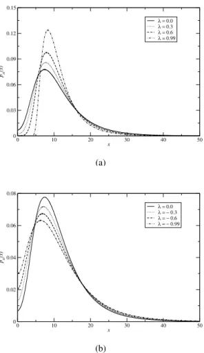
The results of our calculations for the steady state proba-bilitypst(x)as a function of cell number xare presented in
Figs. 1a and 1b. In particular, we have studied the effect of the intensity of correlation strengthλbetween the additive and multiplicative noise intensities onpst(x). It is evident from the
Fig. 1a that with the increase ofλ,pst(x)decreases at smaller xvalues ie,x≤5. However, the peak ofpst(x)increases with
higher values ofλand at higherxvalues,pst(x)for different
λ, merge with each other and die out. This implies that higher values ofλpromote cell growth. In Fig. 1b we have studied the effect of negative correlation strength onpst(x). It is
0 10 20 30 40 50
x
0 0.03 0.06 0.09 0.12 0.15
pst
(x)
λ = 0.0 λ = 0.3 λ = 0.6 λ = 0.99
(a)
0 10 20 30 40 50
x
0 0.02 0.04 0.06 0.08
pst
(x)
λ = 0.0 λ = − 0.3 λ = − 0.6 λ = − 0.99
(b)
FIG. 1: (a) Plot of pst(x)as a function ofxfor different values of
positive correlation parameterλ. We have useda=1,b=0.1,D=
0.3 andα=3.0. (b) Plot of pst(x)as a function ofxfor different
values of negative correlation parameterλ. All other parameters are
same as (a). Parameter values are in arbitrary units.
at smallx, and decreases at largex. This implies that decreas-ingλcauses the tumor cells to disappear. In other words the distribution of the cell population which was mainly peaked about zero (for smaller values ofλ) signifies high extinction rates, and moves towards zero with the decrease of the correla-tion parameterλ. Similar behaviour has also been obtained in the case of logistic growth [19]. Comparing Figs. 1a and 1b, we found that a change in sign concerning the correlation be-tween additive and multiplicative noises has both positive and negative effects on tumor growth. Indeed, a negative value of
λ (which corresponds to a shift to lower values of the peak position of thepst(x)) has a meaning in this context. It
corre-sponds to a change in sign of the correlation between additive and multiplicative noise, which corresponds to a better inter-pretation of the Eq. (4). In fact, in Eq. (4)the additive and multiplicative noise have opposite effects (when one is posi-tive the other is negaposi-tive). Therefore, it seems that a posiposi-tive
λindicates a negative feedback between the two noises. On the contrary a negativeλ, or alternatively a change in sign of either of the two noise terms in Eq.(4), may be correct, to sim-ulate positive feedback of two effects in the tumor treatment.
0 2 4 6 8 10
D
10 12 14
〈
x
〉
α = 0.1, λ = 0.0 α = 0.5 α = 1.0 α = 3.0 α = 5.0 α = 7.0 α = 10.0
FIG. 2: Plot ofxas a function ofDfor different values ofα,λ=
0.0. All other parameter values are the same as Fig. 1.
In Fig. 2, we present our results for average cell population
xas a function of the intensity of multiplicative noiseDfor different values of additive noise intensityαat a fixedλ=0.0. This is given by the equation,
x=
xpst(x)dx
pst(x)dx
. (14)
We observe from Fig. 2 thatx increases first, and then decreases with the intensity of the multiplicative noise, show-ing a typical stochastic resonance characteristic. This means that the appropriate intensity of multiplicative noise is suitable for tumor cell growth and extra noise may restrain tumor cell growth. It is evident from Fig. 2 that asαincreases the peaks die out and become flat. In Fig. 4, we also observe the same qualitative behaviour for the logistic model.
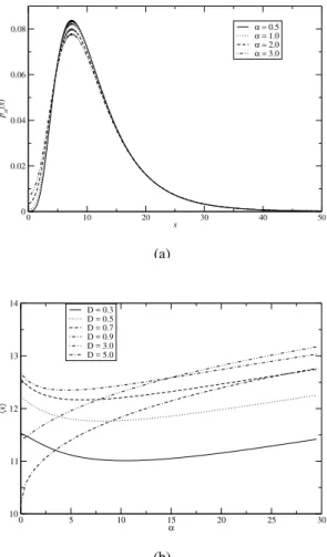
In Fig. 3a we present the results forpst(x)as a function of xat various values ofα. This figure shows that the position of the peaks of the distribution remains unchanged as the inten-sity of the additive noise increases. However, the height of the peaks decrease asαincreases. In Fig. 5a, we also observe the same qualitative behaviour for the logistic model.
or-0 10 20 30 40 50
x
0 0.02 0.04 0.06 0.08
pst
(x)
α = 0.5 α = 1.0 α = 2.0 α = 3.0
(a)
0 5 10 15 20 25 30
α 10
11 12 13 14
〈
x
〉
D = 0.3 D = 0.5 D = 0.7 D = 0.9 D = 3.0 D = 5.0
(b)
FIG. 3: (a) Plot ofpst(x)as a function ofxfor different values ofα.
(b) Plot ofxas a function ofαfor different values ofD. All other
parameter values of both Figs. 3a and 3b are the same as Fig. 1.
der to understand the occurance of stochastic resonance-like phenomena and the underlying mechanism(s) in the present non-bistable systems.
IV. EFFECT OF FINITE CORRELATION TIME ON AVASCULAR TUMOR GROWTH MODELS
In this section we study the stationary properties and av-erage populations of tumor cell growth using the Gompertz and logistic laws in the presence of cross correlated additive and multiplicative noises for the case of nonzero correlated time between noises. This reflects the inclusion of coloured noise into our system and is more appropriate in representing a non-sharp separation of time scales and a greater precision in analysis of the stochastic process. This generalization re-laxes the restriction that the correlation time is zero which is the case when considering Gaussian white noise as in Sec. III above.
0 2 4 6 8 10
D
8 10 12 14 16 18 20
〈
x
〉
α = 0.1, λ = 0.0 α = 0.5 α = 1.0 α = 3.0 α = 5.0 α = 7.0 α = 10.0
FIG. 4: Plot ofxas a function ofDfor different values ofα. All
other parameter values are the same as Fig. 1.
0 10 20 30 40
x
0 0.02 0.04 0.06 0.08
pst
(x)
α=0.5
α=1.0 α=2.0 α=3.0
0 2 4 6 8 10
α
8.4 8.6 8.8 9 9.2 9.4
〈
x
〉
D=0.5 D=0.7 D=1.0 D=0.9
FIG. 5: Plot ofpst(x)as a function ofx(left) for different values ofα
and for fixed values ofD=0.3. Plot ofxas a function ofα(right)
for different values ofD. All other parameter values of Figs. are the
same as Fig. 1.
In modelling the Gompertz and logistic growth laws driven by cross-correlated noises for the case of nonzero correlation time, we implement Eq.(9)instead of Eq.(8)in our proba-bility distribution calculation (Eq. 13).
A. Gompertzian growth
First we study the effect ofλonpst(x)as function ofxfor
a fixed value of correlation timeτ=0.3. This is presented in Fig.6(a). This figure shows that pst(x)as a function ofx
0 10 20 30 40 50
x
0 0.02 0.04 0.06 0.08
pst
(x)
λ = 0.1, τ = 0.3 λ = 0.2 λ = 0.3
(a)
0 10 20 30 40 50
x
0 0.02 0.04 0.06 0.08
pst
(x)
τ = 0.0, λ = 0.2 τ = 0.4 τ = 0.8
(b)
FIG. 6: (a) Plot ofpst(x)as a function ofxfor different values ofλ
atτ=0.3,D=0.3,α=3.0,a=1 andb=0.1. (b) Plot ofpst(x)as a
function ofxfor different values ofτatλ=0.2. All other parameter
values are the same as 6(a). Parameter values are in arbitrary units.
in studying how both the correlation strengthλ and the cor-relation timeτaffect the probability distribution. In Fig. 6b, we present the results of pst(x)as a function ofxfor a fixed
value of correlation strengthλ=0.2 and varying the correla-tion timeτ. As shown in the figure the probability as a func-tion ofxdecreases as we increaseτ. On comparing Figs. 6a and 6b, we find that the correlation strengthλand the correla-tion timeτplay the opposite role on the steady state probabil-ity i.e., pst(x)increases with the increase ofλand decreases
with the increase ofτ.
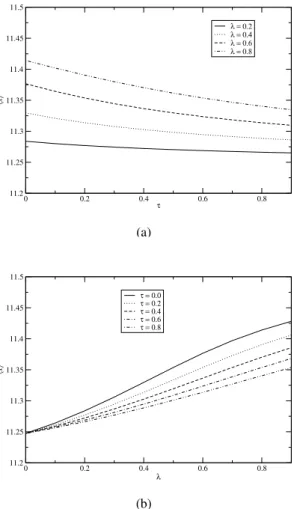
To see the effect ofλandτon the cell population, we ex-amine in Figs. 7a and 7b, the average cell populationx, as a function ofτfor various values ofλand as a function ofλ
for different values ofτ, respectively. From these figures, we observe thatxas a function ofτincreases with increasingλ
and, viewed as a function ofλ, decreases with increasing val-ues ofτ. This also confirms that the correlation strength and the correlation time have the opposite effect on the average cell population in the case of Gompertz growth.
In Fig. 8 we examine the effect of τ on the average cell populationxas a function of additive noise intensityαfor
0 0.2 0.4 0.6 0.8
τ
11.2 11.25 11.3 11.35 11.4 11.45 11.5
〈
x
〉
λ = 0.2 λ = 0.4 λ = 0.6 λ = 0.8
(a)
0 0.2 0.4 0.6 0.8
λ
11.2 11.25 11.3 11.35 11.4 11.45 11.5
〈
x
〉
τ = 0.0 τ = 0.2 τ = 0.4 τ = 0.6 τ = 0.8
(b)
FIG. 7: Plot ofxas a function ofτfor different values ofλ. (b) Plot
ofxas a function ofλfor different values ofτ. All other parameter
values are the same as Fig. 6.
different values of multiplicative noise intensityDat a fixed
λ=0.1. xas a function ofαdecreases for some fixed val-ues ofDand then increases showing a negative resonance-like characteristic and these resonance-like characteristics die out asDis increased. However, there is no change in qualitative nature of the curve with the change inτ, i.e., the correlation time has no effect on the resonance-like characteristic (see left and right figures, these are for differentτ=0.2 and 0.6). Si-miliar results have been obtained for the logistic models.
B. Logistic growth
0 2 4 6 8 10 α 10
10.5 11 11.5 12 12.5 13
〈
x
〉
D = 0.5, λ = 0.1, τ = 0.2
D = 0.7 D = 0.9 D = 1.0 D = 3.0 D = 5.0
0 2 4 6 8 10 10
10.5 11 11.5 12 12.5 13
τ = 0.6
FIG. 8: Plot ofxas a function ofαfor different values ofDat a
fixedλ=0.1. Parameter values are the same in both the left and right
hand figures exceptτ=0.2 (left figure) andτ=0.6 (right figure).
0 10 20 30 40 50
x
0 0.02 0.04 0.06 0.08
pst
(x)
λ = 0.1, τ = 0.3 λ = 0.2 λ = 0.3
(a)
0 10 20 30 40 50
x
0 0.02 0.04 0.06 0.08
pst
(x)
τ = 0.0, λ = 0.2 τ = 0.4 τ = 0.8
(b)
FIG. 9: Same as Fig. 6.
opposite effect onpst(x)contrary to our findings in the present
calculations. The discrepancy between our results and those of [10] in this section are reflected in the fact that [10] have based their model on the original model of [9].
We also studied the effect of nonzero correlation time on average cell population (Figs. 10a and 10b). We observe that
0 0.2 0.4 0.6 0.8
τ 9.6
9.8 10 10.2 10.4 10.6 10.8 11
〈
x
〉
λ = 0.2 λ = 0.4 λ = 0.6 λ = 0.8
(a)
0 0.2 0.4 0.6 0.8
λ 9.6
9.8 10 10.2 10.4 10.6 10.8 11
〈
x
〉
τ = 0.0 τ = 0.2 τ = 0.4 τ = 0.6 τ = 0.8
(b)
FIG. 10: Same as Fig. 7.
0 2 4 6 8 10 α 9.8
10 10.2 10.4 10.6 10.8
〈
x
〉
D = 0.5, λ = 0.1, τ = 0.2
D = 0.7
D = 0.9
D = 1.0
0 2 4 6 8 10 9.6
9.8 10 10.2 10.4 10.6 10.8 11
τ = 0.6
FIG. 11: Same as Fig. 8.
As in the Gompertz model, we study the effect ofτat a fixed
λ=0.1 on the average cell populationxas a functon of ad-ditive noise intensityα for different values of multiplicative noise intensityDin the case of logistic growth model and the results are shown in Fig.11. As one can see these results are analogous to the results obtained in the case of zero correla-tion time in the logistic model and show similar resonance-like characteristics. However, as in the case of Gompertz growth law here we also observe that there is no effect of τ
on the resonance.
V. CONCLUSIONS
We have considered the steady state properties of tumor cell growth, average cell populations and the effect of correlated noise using the Gompertz model. Our results were compared with existing calculations of the logistic model [9, 19] and [10]. In each of the Gompertz and logistic models we found that the both negative and positive correlation between addi-tive and multiplicaaddi-tive noise were important in predicting the likely outcome of treatment protocols. From our results it is also observed that an inappropriate noise intensity can lead to the malignant growth of tumor cells. Another interesting re-sult we found, is that multiplicative noise induces a phase tran-sition and resonance in tumor growth. This behaviour arises due to the sigmoidal nature of both the Gompertz and logistic models which both have points of inflection that are always a fixed proportion of their asymptotic values. It would be in-teresting to pursue this study further, in order to understand the underlying mechanism(s) for the negative stochastic res-onance like characteristic in the Gompertz and logistic
non-bistable models.
We have studied the stationary properties of the Gompertz and logistic tumor cell growth models in the case of nonzero cor-relation time between additive and multiplicative noises. We found that the correlation time and the correlation strength play opposite roles on the steady state probability distribu-tion in case of both the Gompertz and logistic model. As we increased the correlation strength, the steady state probabil-ity and the average cell population increased. This scenario is reversed if the correlation time is increased. Similarly to the case of nonzero correlation time, we observed a phase transi-tion and resonance like characteristics in each of the Gompertz and logistic models. These phenomena are unaffected with the change of correlation time. It is worth mentioning here that in the logistic model we found our calculations significantly differed from those of both [9] and [10]. These results can be reproduced if one considers a negative correlation strength (λ) between additive and multiplicative noise [19, 20]. Fi-nally there were no significant differences in the interpreta-tion of the results between our simulainterpreta-tions for the Gompertz and logistic models. This is probably due to the fact that these growth models belong to the same class of sigmoid function. These results thus provide strong evidence of a universal be-haviour of sigmoid laws which are present in several problems of biological growth.
Acknowledgements
We thank Dr Sahoo for useful discussions. One of us A. Behera acknowledges financial assistance for an APG Studentship awarded by Queen’s University, Belfast. SFC O’Rourke acknowledges current support from the Leverhulme Trust (Grant No. F/00203/K).
[1] L. Gammaitoni, P. Hanggi, P. Jung, and F. Marchesoni, Rev.
Mod. Phys.70, 223 (1998).
[2] Ya. Jia and Jia-rong Li, Phys. Rev. Lett.78, 994 (1997).
[3] A. A. Zaikin, J. Kurths, and L. Schimansky-Geie, Phys. Rev.
Lett.85, 227 (2000).
[4] J. D. Murray, Mathematical Biology I. Springer: Berlin. (2002).
[5] M. Molski and J. Konarski, Phys. Rev. E.68, 021916 (2003).
[6] S. C. Ferreira Jr., M. L. Matrins, and M. J. Vilela, Phy. Rev. E
67, 051914 (2003).
[7] A. Bru, S. Albertos, J. A. Lopez, I. Asenjo-Garcia, and Bru,
Phys. Rev. Lett.92, 238101 (2004).
[8] G. Albano and V. Giorno, J. Theo. Biol.242, 329-336 (2006).
[9] B. Q. Ai, X. J. Wang, G. T. Liu, and L. G. Liu, Phys. Rev. E.
67, 022903 (2003).
[10] D. C. Mei, C. W. Xei, and L. Zhang, Eur. Phys. J. B.41, 107
(2004).
[11] M. Marusic, Z. Bajzer, J. P. Freyer, and S. Vuk-Pavlovic, Cell. Prolif.27, 73 (1994).
[12] G. G. Steel, Basic Clinical Radiobiology. Arnold: third edition. (2002).
[13] M. A. A. Castro, F. Klamt, V. A.Grieneisen, I. Grivicih, and J.
C. F. Moreira, Cell. Prolif.36, 65 (2003).
[14] M. Gyllenberg and G. F. Webb, Growth, Dev. and Aging.53,
25-33 (1989).
[15] A. R. Kansal, S. Torquato, E. A. Chiocca, and T. S. Deisboeck,
J. Theor. Biol.207, 431 (2000).
[16] F. Kozusko and Z. Bajzer, Math. Biosci.185, 153 (2003).
[17] H. Risken, The Fokker-Planck Equation (Springer: Berlin), 96 -99 (1996).
[18] C. W. Gardiner, Handbook of Stochastic Methods. (Spinger: Berlin), 108 - 125 (2003).
[19] A. Behera and S. F. C. O’Rourke, Phys. Rev. E.77, 013901
(2008).
[20] B. Q. Ai, X. J. Wang, and Li. Q. Liu, Phys. Rev. E.77, 013902