Electromagnetic Field Correlators, Maxwell Stress Tensor,
and the Casimir Effect for Parallel Walls
F. C. Santos, J. J. Passos Sobrinho, and A. C. Tort Instituto de F´ısica, Universidade Federal do Rio de Janeiro,
Cidade Universit´aria - Ilha do Fund˜ao - Caixa Postal 68528, 21945-970 Rio de Janeiro RJ, Brazil Received on 23 May, 2005
We evaluate the quantum electromagnetic field correlators associated with the electromagnetic vacuum dis-torted by the presence of two plane parallel conducting walls and in the presence of a conducting wall parallel to a perfectly magnetically permeable one. Regularization is performed through the generalized zeta funtion technique. Results are applied to rederive the atractive and repulsive Casimir effect through Maxwell stress tensor. Surface divergences are shown to cancel out when stresses on both sides of the material surface are taken into account.
I. INTRODUCTION
According to Casimir [1], the (macroscopically) observable vacuum energy of a quantum field is the regularized difference between the zero point energies with and without the external conditions demanded by the particular physical situation at hand. In the case of the quantized electromagnetic field con-fined between two infinite parallel conducting walls separated by a distance a, Casimir’s conception of the vacuum energy leads to a force per unit area between the walls given by
F A =−
π~c
240a4. (1)
Until 1997 only one experiment involving Casimir’s original setup had been performed [2]. Lately, however, the exper-imental observation of this tiny force with metallic surfaces was significantly improved by a series of new experiments due to Lamoreaux, Mohideen and Roy, and Mohideen [3]. The concept of an observable vacuum energy can be extended to all quantum fields and several types of boundary condi-tions and/or applied external fields. An updated review of all these Casimir effects can be found in the monograph by Bor-dag, Mohideen, and Mostepananko [4], but see also, Mostepa-nenko and Trunov, and Plunienet al.[5].
The local approach to the electromagnetic Casimir effect was initiated by Brown and Maclay who calculated the renor-malized stress energy tensor between two parallel perfectly conducting plates by means of Green functions techniques [6]. An interesting approach to the standard Casimir effect is the one due to Gonzales [7]. Analyzing the vacuum oscil-lations of the electromagnetic field confined by two parallel slabs separated by a gap of sizea, Gonzales pointed out that the apparently non-objectionable definition of the vacuum en-ergy given above could easily lead to conceptual errors and stressed the fact that in any Casimir interaction calculation, contributions frombothsides of the material surfaces involved must be taken into account. This is so because the vacuum pressure always pushes the material surfaces involved, there-fore, the repulsiveness or atractiveness of the Casimir force depends on the discontinuity of the relevant component of the quantized Maxwell stress tensor at the location of the surface. The purpose of this paper is to pursue this line of reason-ing by analyzreason-ing the stresses on parallel plane walls due to
the vacuum distortions caused by the presence of these walls through the quantized version of the Maxwell stress tensor. Though the approach chosen here has many points in common with Ref. [7] cited above and Green functions techniques [8], it is a different alternative in the sense that it relies on objects known as correlators, which are regularized vacuum expec-tation values of products of the electromagnetic field compo-nents taken at the same point of space and for equal times. These correlators contain all the information we need about the local behavior of the vacuum expectation values of ele-ments of Maxwell stress tensor, in particular, their behavior near both sides of the material surface in question, a feature crucial to the obtention of the correct result. The local behav-ior of the Maxwell tensor, or of the relativistic symmetrical stress-energy tensor, is extremely important because as shown by, for example, Deutsch and Candelas [9] with the help of Green functions techniques, as we approach the boundaries we find strong divergencies that cannot be simply removed by usual renormalization procedures. Besides reviewing the ob-tention of the electromagnetic Casimir for the standard case of two perfectly conducting parallel walls, we will also consider a pair of parallel walls, one of them perfectly permeable. This setup was first proposed by Boyer [10] who analyzed them from the viewpoint of random electrodymanics and it is the simplest example of a repulsive Casimir force. For both cases, the conducting plate and Boyer’s setup we also construct the symmetrical stress tensor. We will employ Gaussian units and setc=~=1.
II. MAXWELL STRESS TENSOR AND THE
ELECTROMAGNETIC FIELD CORRELATORS
on the location of the walls. The Cartesian components of the Maxwell stress tensor (in Gaussian units) are given by [11]
Ti j= 1 4π
µ
EiEj− 1 2δi jE
2+BiB
j− 1 2δi jB
2
¶
(2)
wherei,j=x,y,z. Suppose that the material surface is placed perpendicularly to the
OZ
axis. Upon quantizing the electro-magnetic field we can write the quantum version of (2). For instance,ˆ
Tzz®0= 1 8π
h
ˆ Ez2
®
0−
D
ˆ Ek2E
0+
ˆ
B2z
®
0−
D
ˆ B2kE
0
i
, (3)
where ˆEk2=Eˆ2
x+Eˆy2and ˆB2k=Bˆ2x+Bˆ2y;
ˆ
O®0≡ h0|Oˆ|0i de-notes a vacuum expectation value. The other Cartesian com-ponents of this tensor can be obtained in an analogous way. The quantum macroscopic forceFˆ®0on the wall can be eval-uated by integrating the quantum version of the classical result [11]
F=
Z
∂R
˜
T·ˆnda, (4)
wereˆnis the outward normal at the boundary∂R and
R
is any region containing all or part of the wall. Classically, (4) can be obtained by integrating the Lorentz force per unit volume acting on charge and current distributions and eliminating the sources in favor of the fields. From a quantum point of view, we see that the problem of evaluating the pressure the material surface due to the distorted zero point oscillations of the elec-tromagnetic field is reduced to the evaluation of the vacuum expectation value of the quantum operators ˆEi(r,t)Ejˆ (r,t),ˆ
Bi(r,t)Bˆj(r,t),and ˆEi(r,t)Bjˆ (r,t). The evaluation of these correlators depends on the specific choice of the boundary conditions. A regularization recipe will also be necessary, for these objects are mathematically ill-defined. For the setup en-volving conducting plates these correlators were evaluated by L¨utken and Ravndal [16], see also [12]. They can be also ob-tained from the coincidence limit of the photon propagator be-tween conducting plates evaluated by Bordaget al[17]. In the next section we will evaluate and regularize these correlators by means of analitycal continuation techniques [13] similar,
though not equal, to the ones employed by L¨utken e Ravn-dal [16]. We will also show how to obtain the corresponding results for another unusual but intersting setup [13].
III. CORRELATORS FOR CASIMIR’S SETUP
Consider an experimental setup consisting in two infinite perfectly conducting parallel plates (ε→∞) kept at a fixed distanceafrom each other. We will choose the coordinates axis in such a way that the
OZ
direction is perpendicular to the plates. One of the plates will be placed atz=0 and the other one atz=a. The field must satisfy the following bound-ary conditions on the plates: the tangential componentsEx e Ey of the electric field and the normal componentBz of the magnetic field must be zero on the plates. Since there are no real charges or currents it will be convenient to work in the Coulomb gauge in which∇·A(r,t) =0, andΦ=0, thus E(r,t) =−∂A(r,t)/∂tandB(r,t) =∇×A(r,t). These phys-ical boundary conditions combined with the choice of gauge allow us to rewrite the boundary conditions in terms of the components of the vector potential A(r,t) in the following way: at z=0 we will have,Ax(x,y,0,t) =0 ; Ay(x,y,0,t) =0 ;
∂
∂zAz(x,y,0,t) =0, (5) and atz=a,
Ax(x,y,a,t) =0 ; Ay(x,y,a,t) =0 ;
∂
∂zAz(x,y,a,t) =0. (6) The vector potential operatorAˆ(r,t) that satisfies the wave equation, the Coulmb gauge and the boundary conditions can be written as
ˆ
A(r,t) = 1
π
³π
a
´12 ∞′′
∑
n=0Z d2κ
√ωnaˆ(1)(κ,n)κˆ×zˆsin³nπz a
´
+ aˆ(2)(κ,n)
·
ˆ κωin
asin
³nπz
a
´
−ˆzκ ωcos
³nπz
a
´¸¾
ei(κ·ρ−ωt) +h.c, (7) whereκ= (kx,ky)andρis the position arrow on the
X Y
plane. The normal frquencies are given byω=ω(κ,n) =
r
κ2+n2π2
a2, (8)
ocupation number space and satisfy
h
ˆ
a(λ)(κ,n),aˆ†(λ′)(κ′,n′)i=δλλ′δnn′δ¡κ−κ′¢. (9) It is convenient to write the vector potential in the general form
ˆ A(r,t) =
∞′′
∑
n=0Z
d2κ 2
∑
λ=1 ˆ
a(λ)(κ,n)A(κλn)(r)e−iω(κ,n)t+h.c, (10)
whereA(κλn)(r)are the modal functions. The modal functions for each polarization state must obey Helmholtz equation and the boundary conditions given above. In our case the modal functions are
A(κ1n)(r) = 1
π
³π
a
´12 1
√ωsin³nπz a
´
e−iκ·ρκˆ×ˆz, (11)
and
A(κ2n() r) =1π³π a
´12 1
√ω
·
ˆ κinπ
aωsin
³nπz
a
´
−ˆzκ ωcos
³nπz
a
´¸
e−iκ·ρ. (12)
The next step is to evaluate the electric field operatorEˆ(r,t). Recalling that ˆa(λ)(κ,n)|0i=0, we first write the correlators <Ei(ˆ r,t)Eˆj(r,t)i0in the general form
<Ei(ˆ r,t)Eˆj(r,t)i0=
∑
α Eiα(
r)E∗jα(r), (13)
where we have introduced the modal functionsEiα(r)for the electric field. In our case (11) and (12) yield
E(i1κ)n(r) =πi
µω
(κ,n)π a
¶12
sin³nπz a
´
e−iκ·ρ(κˆ×ˆz)i, (14)
and,
E(i2κ)n(r) =πi
µω(κ,n)π
a
¶12 ·
κi inπ aω(κ,n)sin
³nπz
a
´
−ˆzi
κ ω(κ,n)cos
³nπz
a
´¸
e−iκ·ρ, (15)
respectively. Taking (14) and (15) into (13), we writeκˆi=cosφδix+sinφδiy,ˆzi=δize(ˆz×κˆ)i=sinφδix−cosφδiy, whereφis the azimuthal angle on the
X Y
plane and we have performed all angular integrals. In this way we end up withhEi(ˆ r,t)Ej(ˆ r,t)i0 =
µ
2 π
¶³π
a
´δki j
2
∞′′
∑
n=0sin2³nπz a
´Z∞
0
dκκω(κ,n)
+
µ
2 π
¶³π
a
´ ³π
a
´2δki j
2
∞′′
∑
n=0n2sin2³nπz a
´Z∞
0 dκκω
−1(κ,n)
+
µ
2 π
¶ ³π
a
´
δ⊥
i j
∞′′
∑
n=0cos2³nπz a
´Z ∞
0 dκκ
3ω−1(κ,n),
(16)
whereδki j:=δixδjx+δiyδjyeδ⊥i j:=δizδjz. Equation (16) is a formal expression for the correlatorhEi(r,t)Ej(r,t)i0, since it is mathematically ill-defined unless a regularization recipe is prescribed. We will regularize the integrals in (16) with the help of analytical continuation methods.
Consider, for instance, the first integral on the r.h.s. of (16) and let us rewrite it as follows
Z∞
0 dκκ
µ
κ2+n2π2 a2
¶1/2
→
Z ∞
0 dκκ
µ
κ2+n2π2 a2
¶1/2−s
.
The first term in (16) can be rewritten as
T1=
µ
2 π
¶³π
a
´δki j
2
∞”
∑
n=0sin2³nπz a
´Z ∞
0 dκκ
µ
κ2+n2π2 a2
¶12−s
the second as
T2=
µ
2 π
¶ ³π
a
´ ³π
a
´2δki j
2
∞”
∑
n=0n2sin2³nπz a
´Z ∞
0 dκκ
µ
κ2+n2π2 a2
¶−12−s
, (18)
and the third one as
T3=
µ
2 π
¶ ³π
a
´
δ⊥
i j
∞”
∑
n=0cos2³nπz a
´Z ∞
0 dκκ
3
µ
κ2+n2π2 a2
¶−12−s
. (19)
Let us assume thatℜsis large enough to give precise mathematical meaning to these integrals. After evaluating them and make use of the analytical continuation of the results we will take the limits→0. Let us see, for instance, what happens withT1. Making use of the following representation of Euler beta function [19]
Z ∞
0 dx x µ−1¡
x2+c2¢ν−1=B 2
³µ
2,1−ν− µ 2
´
cµ+2ν−2, (20)
whereB(x,y) =Γ(x)Γ(y)/Γ(x+y), and that holds forℜ¡ν+µ2¢
<1 andℜµ>0, we obtain
Z∞
0 dκκ
µ
κ2+n2π2 a2
¶1/2−s
=1 2
³nπ
a
´3−2s Γ(s−3/2)
Γ(s−1/2)= 1 (2s−3)
³nπ
a
´3−2s
. (21)
Taking this result intoT1we obtain
T1=
µ
1 2s−3
¶³π
a
´3−2sδki j
2a
"
ζR(2s−3)−
∞
∑
n=0n3−2scos
µ
2nπz a
¶#
, (22)
whereζR(z)is the well-known Riemann zeta function. Taking the limits→0, we have
T1=− 1 3π
³π
a
´4δki j
2
"
1 120+
1 8
∞
∑
n=1d3
dξ3sin(2nξ)
#
, (23)
where we made use of the fact thatζR(−3) =1/120, definedξ:=πz/a, and wrote
n3cos(2nξ) =−1 8×
d3
dξ3sin(2nξ). (24)
The sum on the R.H.S. of (23) can be regularized in many ways. A quick though non-rigorous way is to write
T1=−1 3π
³π
a
´4δki j
2
"
1 120+
1 8
d3 dξ3
∞
∑
n=1sin(2nξ)
#
, (25)
and express the summand in terms of exponential functions of imaginary argument thereby transforming each one of the sums into the euclidean space. In this way we obtain
∞
∑
n=1sin(2nξ) = 1 2i
à ∞
∑
n=1exp(i2nξ)−
∞
∑
n=1exp(−i2nξ)
!
= 1 2i
à ∞
∑
n=1exp(2nξE)−
∞
∑
n=1exp¡
−2nξ′E
¢ !
(26)
where we have made the substitutioniξ→ −ξE in the first sum andiξ→ξ′E in the second. Each one of the sums above
can be easily performed and the result is
∞
∑
n=1sin(2nξ) =1
It follows that
T1=−1 3π
³π
a
´4δki j
2
·
1 120+
1 8
d3 dξ3
1 2cot(ξ)
¸
. (28)
Treating the two other terms in (16) in a similar manner we obtain
T2=−π1³π a
´4δki j
2
·
1 120+
1 8
d3 dξ3
1 2cot(ξ)
¸
, (29)
and
T3= 4 3π
³π
a
´4δ⊥i j
2
·
1 120−
1 8
d3 dξ3
1 2cot(ξ)
¸
. (30)
Notice that some care must be taken when we aply this pro-cedure to the third term. This is so because the term corre-sponding ton=0 inT3is not zero. In fact its contribution is:
T3(n=0) =
µ
2 π
¶³π
a
´
δ⊥
i j
Z∞
0
dκκ−2−2s, (31)
which diverges when the regularization is removed. However this term is non-physical and can be safely ignored. Finally, collecting all partial results we have
hEi(r,t)Ej(r,t)i0 = T1+T2+T3 = ³π
a
´4 2
3π
·³
−δk+δ⊥´ i j
1
120+δi jF(ξ)
¸
. (32)
The functionF(ξ)is defined by
F(ξ):=−1 8
d3 dξ3
1
2cot(ξ), (33)
and its expansion aboutξ=0 is given by
F(ξ)≈3 8ξ
−4+ 1 120+O
¡ξ2¢
. (34)
Nearξ=π(which corresponds toz=a) we make the replacementξ→ξ−π. Notice that due to the behavior ofF(ξ)near ξ=0,a, strong divergences predominate in the behavior of the correlators near the plates.
By applying the exactly the same procedure we obtain the magnetic field correlators
hBi(r,t)Bj(r,t)i0=
³π
a
´4 2
3π
· ³
−δk+δ⊥´ i j
1
120−δi jF(ξ)
¸
. (35)
A direct evaluation also shows that the correlators < Ei(r,t)Bj(r,t)i0are zero.
IV. CORRELATORS FOR BOYER’S SETUP
The other setup we are interested in is that one in which a perfectly conducting plate is placed atz=0 and perfectly per-meable plate is placed atz=a. This setup was analyzed for the first time by Boyer in the contetxt of stochastic
electrody-namic [10] and it is the simplest case of a repulsive Casimir effect that can be found in the literature. The boundary condi-tions now are:(a)the tangential componentsExandEyof the electric field as well as the normal componentBzof the mag-netic field must vanish on the surface of the plate atz=0;(b) the tangential components ofBxeByof the magnetic field as well as normal conponentEzof the electric field must vanish on the surface of the plate atz=a. These boundary conditions translated in terms of the components of the vector potential read
Ax(x,y,0,t) =0 ; Ay(x,y,0,t) =0 ; ∂∂
at z=0, and atz=a
∂
∂zAx(x,y,a,t) =0 ;
∂
∂zAy(x,y,a,t) =0 ; Az(x,y,a,t) =0. (37) The appropriate vector potential operatorAˆ(r,t)is given by [13]
ˆ
A(r,t) = π1³π a
´12 ∞
∑
n=0Z d2κ √ω
½
ˆ
a(1)(κ,n)κˆ×zˆsin
·µ
n+1 2
¶π
z a
¸
+ aˆ(2)(κ,n)
"
ˆ
κi(n+12)
ωa sin
·µ
n+1 2
¶π
z a
¸
−ˆzκ ωcos
·µ
n+1 2
¶π
z a
¸#)
×ei(κ·ρ−ωt) + h.c., (38)
where as beforeκ= (kx,ky)andρis the position vector on the
X Y
plane. The normal frequencies are givenω(κ,n) =
s
κ2+
µ
n+1 2
¶2π2
a2, (39)
withkx,ky∈Randn∈N−1. Notice that contrary to the case of two conducting plates normalization does not require the we multiply the term corresponding ton=0 by 1/2. The electric and magnetic field correlators for Boyer’s setup can be evaluated with the same technique employed before [13]. In fact, it is not hard to convince ourselves that it is sufficient to perform the substitutionn→n+1/2 and follow the same steps as before to obtain
hEi(r,t)Ej(r,t)i0=T1+T2+T3, (40)
where, for example
T1=Γ
¡
s−32¢
Γ¡
s−1 2
¢ ³π
a
´3−2sδki j
2a
( ∞
∑
n=0µ
n+1 2
¶3−2s
1 2
h
1−cos³2(n+1/2)πz a
´i )
, (41)
The termsT2eT1show a similar structure. The main difference with respect to the two conducting plate case is that now we have to deal with the Hurwitz zeta functionζH(z,q)which has a series representation given by [19]
ζH(z,q) =
∞
∑
n=01
(n+q)z, (42)
withℜz>1, andq6=0,−1,−2, ... In our case we must set ζH(2s−3,
1 2) =
∞
∑
n=0µ
n+1 2
¶3−2s
. (43)
It follows that in the limits→0 we have
T1=−³π a
´4 1
3π δk
i j 2
(
ζH
µ
−3,1 2
¶
+
∞
∑
n=0µ
n+1 2
¶3
cos
µ
2
µ
n+1 2
¶π
z a
¶)
. (44)
In the same way we obtain forT2eT1the results
T2=−³π a
´41
π δk
i j 2
(
ζH
µ
−3,1 2
¶
−
∞
∑
n=0µ
n+1 2
¶3
cos
µ
2
µ
n+1 2
¶π
z a
¶)
. (45)
and
T3=³π a
´4 2
3π δ⊥
i j 2
(
ζH
µ
−3,1 2
¶
+
∞
∑
n=0µ
n+1 2
¶3
cos
µ
2
µ
n+1 2
¶π
z a
¶)
Notice that this time we do not have the divergent contribution corresponding ton=0 as in the case of the conducting plates. Adding the three terms we have
ˆ
Ei(r,t)Eˆj(r,t)®
0 =
³π
a
´4 2
3π
½
(−δki j+δ⊥i j)ζH
µ
−3,1 2
¶
+
∞
∑
n=0µ
n+1 2
¶3
cos
µ
2
µ
n+1 2
¶π
z a
¶)
. (47)
The numerical valueζH¡−3,12¢can be obtained from [19]
ζH(−n,q) =−
Bn+1(q)
n+1 , (48)
wheren∈NandBn+1(q)is a Bernoulli polynomial defined
by [19]
Bn(x) = n
∑
p=0n! p!(n−p)!Bpx
n−k,
(49)
whereBpis a Bernoulli number. The relevant polynomial here is:
B4(x) =x4−2x3+x2− 1
30. (50)
WithB4(1/2) = (7/8)×(1/30), it follows thatζH¡−3,12¢= −(7/8)(1/120). The sum can be regularized with the same technique employed before. In fact, we can define the function G(ξ)by
G(ξ) : =
∞
∑
n=0µ
n+1 2
¶3
cos
·
2
µ
n+1 2
¶
ξ¸
= 1 8
∞
∑
n=0(2n+1)3cos[(2n+1)ξ], (51)
where as beforeξ:=zπ/a. We can write
(2n+1)3cos[(2n+1)ξ] =−d 3
dξ3sin[(2n+1)ξ] (52)
and formally we have
G(ξ) =−1 8
d3 dξ3
∞
∑
n=0sin[(2n+1)ξ]. (53)
Writing sin[(2n+1)ξ]in terms of exponentials of imaginary argument and passing to the euclidean space we obtain after some simple manipulations
G(ξ) =−1 8
d3 dξ3
1
2 sin(ξ). (54)
Collecting all partial results we finally obtain for
ˆ
Ei(r,t)Eˆj(r,t)®
0the result
ˆ
Ei(r,t)Eˆj(r,t)®
0=
³π
a
´4 2
3π
" µ
−7 8
¶¡−δk+δ⊥¢
i j
120 +δi jG(ξ)
#
. (55)
Proceeding in the same way in the evaluation ofˆ
Bi(r,t)Bˆj(r,t)®
0we obtain
ˆ
Bi(r,t)Bˆj(r,t)®0=
³π
a
´4 2
3π
"µ
−7 8
¶¡−δk+δ⊥¢
i j
120 −δi jG(ξ)
#
. (56)
Observe that nearξ=0 the functionG(ξ)behaves as
G(ξ) =3 8ξ
−4 −7
8 1 120+O
¡ξ2¢
, (57)
But nearξ=πits behavior is slightly different
G(ξ) =−3 8(ξ−π)
−4 +7
8 1 120+O
h
(ξ−π)2i. (58)
Again, a direct calculation shows thatˆ
Ei(r,t)Bˆj(r,t)®
Z'
z=0 z=a
ε
z=l
ε,µ ε,µ
Z
n'=-z n=z
^ ^ ^ ^
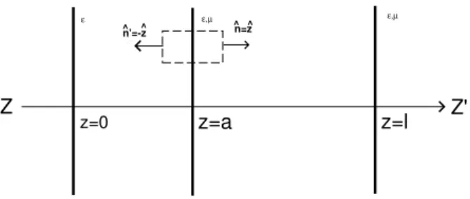
FIG. 1: Three-plate setup for the obtention of the Casimir force per unit area. The plate atz=ℓis auxiliary.
As before the divergent behavior of the correlators near the plates we are interested in is an effect of the distortions of the electromagnetic oscillations with respect to a situation where the plates are not present. This fact has received the attention of several authors, see for example [9, 16].
V. THE CASIMIR EFFECT FOR CONDUCTING PLATES
In order to apply the above results to Casimir’s original setup we consider for convenience three parallel perfectly conducting plates perpendicular to the
OZ
axis atz=0,z=a andz=ℓ.The quantum version of Maxwell tensor is
4πTi jˆ ®0=ˆ
EiEˆj®0−1 2δi j
ˆ
E2®0+ˆ
BiBˆj®0−1 2δi j
ˆ
B2®0 (59)
Making use of the correlator given by (32) we obtain the following partial results
ˆ
Ex2(z,t)®
0=
ˆ
Ey2(z,t®
0=
³π
a
´4 2
3π
·
− 1
120+F(ξ)
¸
, (60)
ˆ
Ez2(z,t
®
0=
³π
a
´4 2
3π
·
1
120+F(ξ)
¸
, (61)
alsoˆ
Ex(z,t)Ey(z,ˆ t)®
0=
ˆ
Ex(z,t)Ez(z,t)ˆ ®
0=
ˆ
Ey(z,t)Ez(z,ˆ t)®
0=0. In the same way, making use of (35) we obtain
ˆ
B2x(z,t)®
0=
ˆ
B2y(z,t®
0=
³π
a
´4 2
3π
·
− 1
120−F(ξ)
¸
, (62)
ˆ
B2z(z,t
®
0=
³π
a
´4 2
3π
·
1
120−F(ξ)
¸
, (63)
and alsoˆ
Bx(z,t)By(z,t)ˆ ®
0=
ˆ
Bx(z,t)Bz(z,t)ˆ ®
0=
ˆ
By(z,t)Bz(z,tˆ )®
0=0. The components of the quantum version of Maxwell tensor can be easily evaluated. For instance
8πTzz(z,t)ˆ ®
0 =
ˆ
Ez2(z,t)
®
0−
ˆ
Ex2(z,t)
®
0−
ˆ
Ey2(z,t)
®
0 +ˆ
B2z(z,t)
®
0−
ˆ
B2x(z,t)
®
0−
ˆ
B2y(z,t)
®
0. (64)
performing the necessary substitutions we have
ˆ
Tzz®
0=
π2
240a4. (65)
In the same way
ˆ
Txx®
0 =
ˆ
Tyy®
0=−
1 8π
¡ˆ
Ez2(z,t)®
0+
ˆ
B2z(z,t)®
0
¢
= − π 2
720a4 (66)
Let us obtain now the Casimir force per unit area between the conducting plates. Consider Figure (V) and the plate at z=a. The Casimir force per unit area on this plate is
Fz
A = −Tzz(z→a
L) +Tzz(z →aR) = − π
2
240a4+
π2
240(ℓ−a)4, (67)
wherez→aL,R means that ztends to a from the left/right. Taking the limitℓ→∞we obtain the expected result for the Casimir force per unit area
Fz A =−
π2
240a4. (68)
The minus sign shows that the resulting pressure pushes to-wards the region between the plates. If simultaneously we take the limitsℓ,a→∞keeping the distanceℓ−aconstant. The pressure changes its sign but it still pushes the plate at z=atowards the one atz=ℓ.
In order to calculate the renormalized symmetrical stress-energy tensor hΘˆµν(z)iren
0 we evaluate the energy density
ρ(z) ≡ hΘˆ00(z)iren
0 in the region between the plates as well as the saptial componentshΘˆxx(z)iren
0 ,hΘˆyy(z)iren0 , and hΘˆzz(z)iren
0 . The energy density is given by
ρ(r,t) = 1 8π
¡ˆ
E2(r,t)®
0+
ˆ
B2(r,t)®
0
¢
(69)
making use of the correlators given by (32) and (35) we obtain
ρ(a) =− π 2
720a4. (70)
This result is due to the fact that the divergent pieces in (32) and (35) cancel out yielding a finite result for the vacuum en-ergy density. Recalling thatΘi j(z) =−Ti j(z), see [11], with help of (2), (32) and (35) the remanescent components of the symmetrical stress-energy tensor are easily obtained. The fi-nal result is
hΘˆµν(z) iren
0 =
π2
720a4diag(−1,1,1,−3), (71) which is in perfect agreement with Brown and Maclay’s re-sults [6]. Notice also that hΘˆµ
µ(z)iren
0 =gµνhΘˆµν(z)iren0 =0, withgµν=diag(1,−1,−1,−1).
VI. THE CASIMIR EFFECT FOR ONE CONDUCTING
PLATE AND AN INFINITELY PERMEABLE ONE
Let us consider now the setup proposed by Boyer [10] which consists of a perfectly conducting plate placed perpen-dicularly to the
OZ
axis atz=0 and another infinitely per-meable one parallel to the first placed atz=a. The boundary conditions on the conducting plate are as beforeEx=Ey=0 andBz=0, and for the infinitely permeable plate:Bx=By=0andEz=0. Making use of the correlator given by (55) the fol-lowing partial results:
ˆ
Ex2(z,t)
®
0=
ˆ
Ey2(z,t
®
0=
³π
a
´4 2
3π
·
7 8×
1
120+G(ξ)
¸
,
(72)
ˆ
Ez2(z,t
®
0=
³π
a
´4 2
3π
·µ
−7 8
¶
× 1
120+G(ξ)
¸
, (73)
and Ex(z,ˆ t)Ey(z,t)ˆ ®
0 =
ˆ
Ex(z,t)Ez(z,ˆ t)®
0 =
ˆ
Ey(z,t)Ez(z,ˆ t)®
0 = 0. By the same token making use of the correlator given by (56) we obtain
ˆ
B2x(z,t)
®
0=
ˆ
B2y(z,t
®
0=
³π
a
´4 2
3π
·
7 8×
1
120−G(ξ)
¸
,
(74)
ˆ
B2z(z,t
®
0=
³π
a
´4 2
3π
·µ
−7 8
¶
× 1
120−G(ξ)
¸
, (75)
and also
ˆ
Bx(z,t)By(z,tˆ )®
0=
ˆ
Bx(z,t)Bz(z,t)ˆ ®
0=
ˆ
By(z,t)Bz(z,t)ˆ ®
0=0 (76) Proceeding as in the case of the conducting plates we obtain the following results for the componenets of the quantum ver-sion of Maxwell tensor
ˆ
Txx®
0=
ˆ
Tyy®
0=
7 8×
π2
720a4, (77)
and
ˆ
Tzz®
0=
µ
−7 8
¶
× π
2
240a4. (78)
Notice that it is sufficient to multiply the results obtained for Casimir’s setup by the factor(−7/8)in order to obtain the results corresponding to Boyer’s setup.
In order to obtain the Casimir force per unit area for this setup it is convenient to place a third conducting plate atz=ℓ. Then the Casimir force per unit area on the plate atz=awill be given by
Fz
A = −Tzz(z→a
L) +Tzz(z →aR) = −
µ
−7 8
¶
× π
2
240a4+
µ
−7 8
¶
× π
2
240(ℓ−a)4.(79) Taking the limit ℓ→∞ we obtain a Casimir force which pushes the plate atz=atowards the regionz>agiven by
Fz A =
7 8×
π2
240a4 (80)
In order to evaluate the symmetrical stress-energy tensor we first evaluate the Casimir energy density. Making use of (55) e (56) we have
ρ=7 8×
π2
240a4. (81)
As in the case of the conducting plates a simple calculation shows that the stress energy tensor for Boyer’s setup is given by
hΘˆµν(z)iren
0 =
7 8 ×
π2
720a4diag(1,−1,−1,3). (82) As beforehΘˆµµ(z)iren
0 =gµνhΘˆµν(z)iren0 =0.
VII. CONCLUSIONS
In this paper we have shown how to employ the equal time and space electromagnetic field correlators evaluated be-tween parallel material surfaces to rederive results concernig
the Casimir energy and pressure and the symmetrical trace-less stress energy tensor. We have shown that for the cases we had in mind here finite results are obtained only when we consider what happens on both sides of the surface boundary. This consideration provided the mechanism by which precise cancellations occurred and finite results were obtained. These cancellations occur only for the simple geometry considered in this paper. This is in agreement with, for example, Ref. [9] and should be considered as a concrete example of the behav-ior of quantized fields near and on boundary surfaces. This behavior depends on the geometry of the boundaries and can become quite complicated. It can depend on the local curva-ture of the boundary, for instance. Finally, it must be men-tioned that the equal time and space electromagnetic field cor-relators calculated here were can be also employed to rederive the atractive and the repulsive Casimir effect by means of a quantum version of the Lorentz force [20]. They can be also applied to the Casimir-Polder interaction between an atom and material surfaces [21]
[1] H. B. G. Casimir, Proc. K. Ned. Akad. Wet. 51, 793 (1948); Philips Res. Rep. 6. 162 (1951).
[2] M. J. Sparnaay, Physica24, 751 (1958).
[3] S. K. Lamoreaux, Phys. Rev. Lett.78, 5 (1997); erratum Phys. Rev. Lett. 81, 5475 (1988); U. Mohideen and A. Roy, Phys. Rev. Lett.81, 4549 (1998).
[4] M. Bordag, U. Mohideen and V.M. Mostepanenko, Phys. Rep.
353, 1 (2001); quant-ph/0106045.
[5] V. M. Mostepanenko and N. N. Trunov, Sov. Phys. Usp. 31, 965 (1988); V. M. Mostepanenko and N. N. Trunov, The Casimir Effect and its Applications, (Oxford, Clarendon, 1997); G. Plu-nien, B. M¨uller and W. Greiner, Phys. Rep. 134, 664 (1987); S. K. Lamoreaux, Am. J. Phys.67, 850 (1999).See also: M.V. Cougo-Pinto, C. Farina and A. C. Tort, Rev. Bras. Ens. F´ıs.22, 122 (2000) (in Portuguese).
[6] L.S. Brown and G.J. Maclay, Phys. Rev.184, 1272 (1969). [7] A. E. Gonzales, Physica131A 228-236 (1985).
[8] K. A. Milton,The Casimir Effect: Physical Manifestations of Zero-Point Energy(World Scientific, Singapore, 2001). [9] D. Deutsch and P. Candelas, Phys. Rev. D20, 3063 (1979). [10] T.H. Boyer Phys. Rev. A9, 2078 (1974).
[11] J. D. Jackson,Classical Electrodynamics, 3rd. ed., (John Wiley, New York 1999).
[12] G. Barton, Phys. Lett. B237, 559 (1990).
[13] M. V. Cougo-Pinto, C. Farina , F. C. Santos and A. C. Tort: J. of Phys. A32(1999), 4463.
[14] H.B.G. Casimir,J. Chim. Phys.46, 407 (1948). [15] T.H. Boyer, Phys. Rev.180, 19 (1969).
[16] C.A. L¨utken and F. Ravndal, Phys. Rev. A31, 2082 (1985). [17] M. Bordag, D. Robaschik and E. Wieczorek, Ann. Phys. (NY)
165, 192 (1985).
[18] E. Elizalde, S. D. Odintsov, A. Romeo, A. A. Bytsenko and S. Zerbini: Zeta Regularization Techniques with Applications, World Scientific, Singapore (1994).See alsoR. Ruggiero, A. H. Zimerman and A. Villani, Rev. Bras. F´ıs.7, 663 (1977). For a simple introduction to the Zeta function regularization tech-nique see: J. J. Passos Sobrinho and A. C. Tort, Rev. Bras. Ens. F´ıs.23, 401 (2001) (in Portuguese).
[19] I. S. Gradshteyn and I. M. Ryzhik,Tables of Integrals, Series and Products, 5th Edition, Academic Press, New York (1994). [20] C. Farina, F. C. Santos and A. C. Tort, Eur. J. of Phys.24N5-N9
(2003).