Brazilian Journal of Physics, vol. 35, no. 3A, September, 2005 641
Two-Body Relationship Between the Pearson-Takai-Halicioglu-Tiller and the
Biswas-Hamann Potential Functions
Teik–Cheng Lim
Nanoscience and Nanotechnology Initiative, Faculty of Engineering,
9 Engineering Drive 1, National University of Singapore, S 117576, Republic of Singapore Received on 6 May, 2005
An approximate and a good parametric relationship between the Pearson-Takai-Halicioglu-Tiller (PTHT) and the Biswas-Hamann (BH) empirical potential energy functions is developed for the case of 2-body inter-action. The approximate relationship between PTHT and BH was obtained by equating the zeroth up to the second order of the potential functions’ derivative with respect to the interatomic distance at the equilibrium bond length, followed by comparison of coefficients at the repulsive and attractive terms. A refined relationship was then suggested by including the third order derivative. Plots of non-dimensional 2-body energy versus the non-dimensional interatomic distance verified the analytical relationships developed herein. Finally, the phys-ical significance of the developed parametric relationships is discussed with reference to conservative design methodology.
I. INTRODUCTION
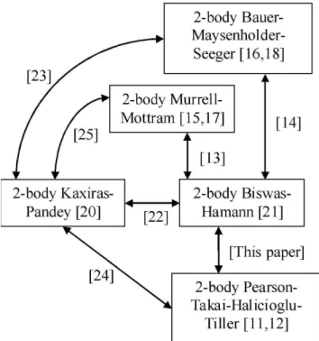
Parametric relationships between various interatomic po-tential energy function of the same category of n-body inter-action can be useful when available physical data and com-putational softwares are based on parameters of different po-tential functions. In addition to providing a way for convert-ing potential functions, any discrepancy between these po-tential functions will provide insight on how the choice of potential functions will affect the outcome of simulation re-sults. Mathematical relationships for relating molecular po-tential functions used in chemical computation have been de-veloped [1-7]. These relationships were improved and sub-sequently developed into a molecular potential function con-verter software [8]. However, parametric relationships be-tween potential energy functions used for computational con-densed matter properties are lacking. Though Stoneham et al. [9] performed a comparison of eight potential functions for silicon, the functions considered are under the category of valence-force potentials which are useful only for describ-ing small distortions from equilibrium. A set of six potential functions were compared by Balamane et al. [10] but the po-tential functions plotted were based on parameters obtained via experimental curve-fitting instead of analytical conversion of parameters. In this paper, a set of analytical relationship is developed for converting parameters between the 2-body in-teractions in the Pearson-Takai-Halicioglu-Tiller (PTHT) and the Biswas-Hamann (BH) potential functions. The PTHT potential function was initially developed for silicon [11], whereby its 2-body energy is taken from the Lennard-Jones potential [12]. The terminology selected here is the “2-body portion of PTHT” instead of “Lennard-Jones” to conform to previous work [13,14], whereby the phrases “2-body portion of Murrell-Mottram” (MM) [15] and the “2-body portion of Bauer-Maysenholder-Seeger” (BMS) [16] were adopted in-stead of the original terms “Rydberg” [17] and “Buckingham” [18] potentials respectively, due to the emphasis for applica-tion in many-body potentials used in condensed matter com-putation [19]. See also Fig.1 whereby the parametric connec-tions amongst the 2-body potential funcconnec-tions of PTHT [11],
MM [15], BMS [16], Kaxiras-Pandey (KP) [20] and BH [21] were connected.
FIG. 1: Recently established relationships and presently developed relationship.
II. ANALYSIS
642 Teik–Cheng Lim
Φ=φ2−body+φ3−body=
∑
i<jUi j+
∑
i<j<kWi jk. (1)
In addition, the 2-body interactions in PTHT and BH be-long to a sub-category of potential function which consist of two distinct parts: a repulsive term and an attractive term,
Ui j=Ui jrepul+Ui jattract. (2) Specifically, the PTHT and BH potential functions for 2-body interactions are written as
UPT HT =ε "µ R r ¶12 −2 µ R r
¶6#
(3)
and
UBH=A1exp(−λ1r) +A2exp(−λ2r) (4) respectively, whereεis the magnitude of the minimum well-depth, r is the interatomic distance and R is the distance at equilibrium for the case of PTHT whilst Ai are the coeffi-cients andλiare the indices of the repulsive(i=1)and attrac-tive(i=2)terms. Furthermore, we note that both the 2-body potentials are such that the functional forms in the repulsive and attractive terms are similar for each potential function, i.e. ε(R/r)6ifor PTHT and A
iexp(−λir)for BH, whereby i=1,2. Let
µ∂nU BH ∂rn
r=R
=
µ∂nU PT HT ∂rn
r=R
(5)
for n=0,1,2,3, we have
ξ0 1 ξ02 ξ1
1 ξ12 ξ2
1 ξ22 ξ3
1 ξ32
½
exp(−ξ1)
exp(−ξ2)
¾ =ε −1 0 72 1512 (6) where
ξi=λiR ; (i=1,2) (7) are the scaling factors. Eliminating the terms Aiexp(−ξi)for
i=1,2 from Eq.(6), we arrive at the upper and lower solutions of one scaling factor in terms of another scaling factor,
½ξ+ i ξ− i ¾ = ½ ξ j
(72/ξj) ¾
. (8)
Solving the first two rows of Eq.(6) simultaneously,
Ai=ε
µ ξ
j ξi−ξj
exp(ξi). (9)
Equation (9) enables the 2-body BH potential, i.e. Eq.(4), to be rewritten in a loose form
UBH=ε
·µ ξ
2 ξ1−ξ2
exp³ξ1
³
1−r R
´´ −
µ ξ
1 ξ1−ξ2
exp³ξ2
³
1−r R
´´¸
, (10)
thereby signifying that the upper solution of Eq.(8) to be in-valid. An approximate relation between PTHT and BH can be obtained by comparing the coefficients of Eq.(10) with those of Eq.(3) to give
ξ1=2ξ2. (11)
Substituting Eq.(11) into the lower solution in Eq.(8), we haveξ1=12 andξ2=6. For attaining better accuracy, we eliminate the terms Aiexp(−ξi)for i=1,2 by solving the last three rows of Eq.(6) to give
ξ1+ξ2=21. (12)
From Eq.(12) and the lower solution of Eq.(8), we obtain
½ξ 1 ξ2 ¾ =1 2 ½
21+√153 21−√153
¾
. (13)
III. RESULTS AND DISCUSSION
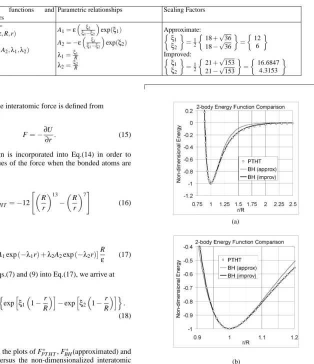
A summary of 2-body interaction relationship between the parameters of PTHT and BH is furnished in Table 1. For verification, graphs of non-dimensional 2-body energy(U/ε) were plotted against the non-dimensional bond length(r/R). Figure 2(a) depicts the approximate and improved BH curves based on PTHT parameters. A close-up view at the minimum well depth is shown in Fig. 2(b). For both illustrations, the developed approximate and a good relationship between the 2-body energy of the PTHT and the BH potential functions has been shown to be valid. It is concluded herein that by con-sidering higher derivative (3rd order), we obtain a much im-proved matching in comparison to the consideration of lower derivative (2ndorder).
In addition to gaining insight on the connection between these potential functions, the parametric relationships also en-able the discrepancies to be clearly observed [26], thereby paving a way for the conservative design methodology to be developed. To further appreciate the physical implications of the relationships furnished in Table 1, we introduce the non-dimensionalized interatomic force as
F∗=
Brazilian Journal of Physics, vol. 35, no. 3A, September, 2005 643
Table 1. Summary of 2-body relationship between PTHT and BH potential function parameters.
Potential functions and parameters
Parametric relationships Scaling Factors
UPT HT= UPT HT(ε,R,r) UBH=
UBH(A1,A2,λ1,λ2)
A1=ε
³ ξ
2 ξ1−ξ2
´ exp(ξ1)
A2=−ε
³ ξ
1 ξ1−ξ2
´ exp(ξ2)
λ1=ξR1
λ2=ξR2
Approximate: ½
ξ1
ξ2
¾
=1
2
½
18+√36 18−√36
¾ =
½ 12
6 ¾
Improved: ½
ξ1
ξ2
¾
=12
½
21+√153 21−√153
¾ =
½ 16.6847
4.3153 ¾
where the absolute interatomic force is defined from
F=−∂∂Ur. (15)
A negative sign is incorporated into Eq.(14) in order to give positive values of the force when the bonded atoms are stretched. Hence
F∗
PT HT =−12 "
µR
r
¶13 −
µR
r
¶7#
(16)
and
F∗
BH=−[λ1A1exp(−λ1r) +λ2A2exp(−λ2r)] R
ε (17)
Substituting Eqs.(7) and (9) into Eq.(17), we arrive at
F∗
BH= ξ1ξ2 ξ2−ξ1
n
exphξ1
³
1−r R
´i −exp
h
ξ2
³
1−r R
´io
.
(18)
Figure 3 shows the plots of F∗
PT HT, FBH∗ (approximated) and
F∗
BH(improved) versus the non-dimensionalized interatomic distance. The approximated and improved F∗
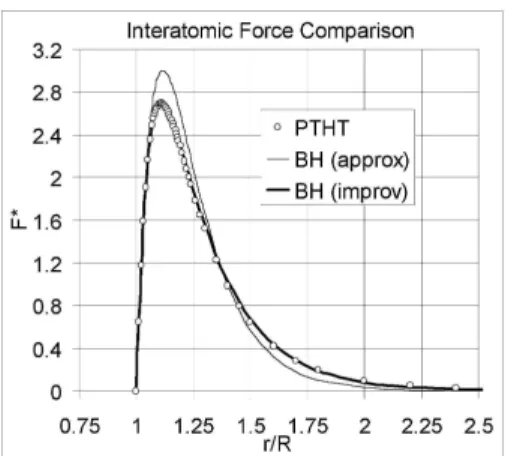
BH are based on the values of the scaling factors shown in Table 1. The higher peak for BH(approx) in Fig. 3 corresponds to the higher slope of the BH(approx) inflexion point in Fig. 2(a) in com-parison to PTHT. We also note that the occurrence of the peak occurs first for BH(approx) in Fig. 3 because the in-flexion point occurs first for BH(approx) in Fig. 2(a). Pre-scription of F∗∈[2.69,3.00] would give simulation results which predicts bond dissociation based on PTHT but no dis-sociation based on BH(approx). However, prescription of (r/R)∈[1.110,1.115] would lead to simulated bond disso-ciation based on BH(approx) but no dissodisso-ciation based on PTHT. Whilst the deviation of BH(approx) from PTHT is about 11.5% at the peak force, the deviation of BH(improv) from PTHT is about 0.1%.
(a)
(b)
FIG. 2: Comparison of 2-body energy function according to PTHT and BH curves (a) long range view, and (b) close up view at minimum well depth.
IV. CONCLUSIONS AND RECOMMENDATION
644 Teik–Cheng Lim
FIG. 3: Comparison of interatomic force of PTHT and BH.
BH potential is more suitable for hard bonds whilst PTHT is more suitable for soft bonds. Note that the bond hardness is different from a strong bond in that the former is a description of the abruptness in the rise of interatomic energy with inter-atomic distance whilst the latter the magnitude of the mini-mum well-depth.
It follows that PTHT is advisable when load is prescribed whilst BH is advisable when distortion is prescribed for con-servative design.
In view of the excellent agreement between parameters of the PTHT and BH(improv) potential functions, a set of rela-tionships between parameters the 3-body energy portion for these two potential functions is suggested for future work.
[1] T.C. Lim, J. Math. Chem. 33, 279 (2003). [2] T.C. Lim, J. Math. Chem. 34, 221 (2003). [3] T.C. Lim, J. Math. Chem. 36, 139 (2004). [4] T.C. Lim, J. Math. Chem. 36, 147 (2004). [5] T.C. Lim, J. Math. Chem. 36, 261 (2004). [6] T.C. Lim, Z. Naturforsch. A 58, 615 (2003).
[7] T.C. Lim, MATCH Commun. Math. Comput. Chem. 49, 155 (2003).
[8] T.C. Lim, MATCH Commun. Math. Comput. Chem. 50, 185 (2004).
[9] A.M. Stoneham, V.T.B. Torres, P.M. Masri, and H.R. Schober, Phil. Mag. A 58, 93 (1988).
[10] H. Balamane, T. Halicioglu, and W.A. Tiller, Phys. Rev. B 46, 2250 (1992).
[11] E. Pearson, T. Takai, T. Halicioglu, and W.A. Tiller, J. Cryst. Growth 70, 33 (1984).
[12] J.E. Lennard-Jones, Proc. Roy. Soc. Lond. A 106, 463 (1924).
[13] T.C. Lim, Z. Naturforsch. A 59, 116 (2004). [14] T.C. Lim, Czech. J. Phys. 54, 553 (2004).
[15] J.N. Murrell and R.E. Mottram, Mol. Phys. 69, 571 (1990). [16] R. Bauer, W. Maysenholder, and A. Seeger, Phys. Lett. A 90,
55 (1982).
[17] R. Rydberg, Z. Phys. 73, 376 (1931).
[18] R.A. Buckingham, Proc. Roy. Soc. Lond. A 168, 264 (1938). [19] S. Erkoc, Phys. Rep. 278, 79 (1997).
[20] E. Kaxiras and K.C. Pandey, Phys. Rev. B 38, 12736 (1988). [21] R. Biswas and D.R. Hamann, Phys. Rev. Lett. 55, 2001 (1985). [22] T.C. Lim, Czech. J. Phys. 54, 947 (2004).
[23] T.C. Lim, MATCH Commun. Math. Comput. Chem. 54, 29 (2005).