Vol. 2 No. 3 pp. 33-44
33
ACREAGE RESPONSE ANALYSIS OF MAIZE GROWERS IN
KHYBER PAKHTUNKHWA, PAKISTAN
B akht aw ar Ri az
Department of Agricultural & Applied Economics, The University of Agriculture,
Peshawar-Pakistan, Email: Bakhtawar_riaz92@hotmail.com
Shahi d Al i
Department of Agricultural & Applied Economics, The University of Agriculture,
Peshawar-Pakistan
Daw ood Ja n
Department of Agricultural & Applied Economics, The University of Agriculture,
Peshawar-Pakistan
Abstract
This study was conducted to analyze the acreage response of maize with respect to price and non-price factors in Khyber Pakhtunkhwa. The time-series data for the period of 35 years (1976-2010) pertaining to, maize area, maize price, rice price, maize yield, average rainfall were collected from various published sources. Nerlovian adjustment lag model and Vector Auto Regression (VAR) technique of estimation was employed for analyzing acreage response of maize. The model explained more than 90 percent of variation in the dependent variable. The expected maize price was unlikely found to be negative and statistically insignificant. The regression coefficients for lag rice price and lag maize yield also appeared insignificant. Area under maize in lagged year was found to be an important variable influencing farmer’s decision on acreage allocation. Among the short run and long run elasticities with respect to lag area that is 0.7155 and 2.5149, long run elasticity was more, signaling that acreage adjustment would normally take place in the long run. The coefficient of lag rainfall was found to be negative and significant indicating a negative relation between maize acreage and rainfall. The short run elasticity of maize area with respect to lag rainfall during the study period has been calculated at -0.0894 while the long run elasticity comes to be -0.3142, indicate its inelastic nature and little effect on the decision of farmers regarding allocation of land to maize. Small area adjustment coefficient (0.2845) revealed low rate of farmers’ area adjustment to desired level because of more institutional and technological constraints. Based upon the findings of this study it can be concluded that farmers allocate land to maize crop mainly basing on their previous allocation pattern rather than relative crop prices.
Key words: Acreage response, Vector auto regression, Short and long run elasticities, maize, Pakistan
1. Introductıon
34
world’s harvest; other top producing countries in 2012 include China, Brazil, Argentina, Mexico, India, Ukraine, Indonesia, France and South Africa. USA produced 273.832 million tones, China 208.258 million tones, Brazil 71.296 million tones (FAOSTAT, 2012).
Maize being the highest yielding cereal crop in the world is of significant importance for countries like Pakistan, where rapidly increasing population, food and fodder demand have already out stripped the available food, feed and fodder supplies. Maize in Pakistan is cultivated as multipurpose food and forage crop, generally by resource poor farmers using marginal land. Maize is currently the leading world cereal both in terms of production and productivity. Maize is an important crop in Pakistan in terms of its food for human, feed for poultry and fodder for livestock utilization and as a raw material for the industry. It is planted on an area of 0.974 million hectare for grain purpose giving an annual production of 3.707 million tones of grains with average yield of 3805 kg/ha. The bulk (97%) of the total production comes from two major provinces, Khyber Pakhtunkhwa and Punjab. Khyber Pakhtunkhwa accounts for 57% of the total area and 68% of total production while Punjab contributes 38% acreage with 30% of total maize grain production. Very little maize (2-3%) is produced in the provinces of Sindh and Balochistan (PARC, 2013).
Maize is the second major cereal crop after wheat in the Khyber Pakhtunkhwa, province of Pakistan, but its yield per unit area is very low. Maize is grown in Kharif season and has the highest yield among all food crops. Its importance for a food-deficient province cannot be over-emphasized. In 2001-2012 total area under maize crop in Pakistan was 944.1 thousand hectare and its yield was 1741 kg/ha. Out of which KPK contribution in area was 536.5 thousand hectare, more than Punjab contribution that is 397.4 thousand hectare. But yield in Punjab i.e. 1883 kg/ha was more than that of KPK, 1655 kg/ha). On the other hand Sindh and Baluchistan contribution was least both in area and yield. In 2010-11, total area under maize was found 974.2 thousand hectare and its yield 3805 kg/ha in which Punjab contributed 534.6 thousand hectare in area and 5444 kg/ha in yield. Khyber Pakhtunkhwa contribution in area was 422.9 thousand hectare and in yield it was 1751 kg/ha (GoP, 2011).
A considerable number of studies have focused on agricultural supply response to price and non-price factors with wide range of crops over the years. More important, expanding cultivated area is a viable option for increasing production (Molua, 2010). Understanding how producers make decisions to allot acreage among crops and how decisions about land use are affected by changes in prices and their volatility is fundamental for predicting the supply of staple crops and, hence, assessing the global food supply situation (Haile et al. 2013).
The production decisions of farmers are dependent on various policies of the government. Price policy, among the others, is the most important one. That is, farmers would allocate their limited land resources to that crop enterprise towards which the relative price movements tend to be favourable. This is however, quite logical and rational as the allocation of land to a better-priced crop would fetch more revenue to farmers. Responsiveness of farmers to economic incentives such as price could influence contribution of agriculture to economy (Mushtaq & Dawson, 2002).
35
The crucial factors responsible for farmers’ area allocation behavior are expected price (based on previous years price), price of competing crop, yield, weather climatic conditions, area, technology etc. The pioneering work of Nerlove (1958) on supply response enables one to determine short run and long run elasticities; also it gives the flexibility to introduce non-price shift variables along with non-price.Very little analytic research as per the knowlede of this researcher has been carried out on acreage response of maize growers in Pakistan (Mushtaq & Dawson, 2002; Nosheen & Iqbal, 2008).Thus there is an intense need to study acreage response of maize growers to price and non-price factors in Khyber Pakhtunkhwa to give an insight to policy makers for allocation of land and production of maize in this province particularly and Pakistan in general.
Acreage response to price and non-price incentives is of considerable importance for devising suitable policy and planning development programmes for the agricultural sector of an economy. Moreover, reliable estimates of acreage response of maize growers are of greater importance for predicting accurately the farmers’ responsiveness towards the price and non price factors and for formulating programmes consistent with national requirement of food and fodder. This study is important because it will assist policy analysts in managing area allocation to maize in this province. The following objectives were set for this study.
To estimate acreage response of maize growers in Khyber Pakhtunkhwa from 1976 to 2010.
To quantify and compare short and long run elasticities of price and non price factors acreage response of maize in Khyber Pakhtunkhwa from 1976 to 2010.
The remainder of this paper is organized into three sections. Section 2 is devoted to data and methodology. Section 3 presents, results and discussion. Section 4 concludes this study with some recommendations.
2. Data and Methodology
This study was conducted in whole Khyber Pakhtunkhwa province. Data for the identified variables was collected from various published sources. Data regarding maize yield was obtained from Agriculture Statistics of Pakistan, and that of prices obtained from Provincial Federal Bureau of Statistics Peshawar for the years 1976 to 2010. Data on rainfall was collected from Pakistan Metrological Department (Peshawar). The data was analyzed via Shazam and Stata (12 version) softwares. The following techniques from simple means to the use of econometric modeling applied for data analysis. The Durbin h statistic (Shazam), Augmented Dickey Fuller test and Vector auto regression was performed (Stata).
Nerlove (1958) introduced the idea of partial adjustment suggesting that since it takes a while for equilibrium to occur, therefore only a partial adjustment takes place within a unit time period. The delay occurring in the equilibrium could be due to many reasons including consumer preferences, which takes a while to change; production already took place and needs to be disposed off.
2.1 Conceptual model
36
Area cultivated in the current time period ( ) is determined by the price expected in the current time period ( ), expected yield period ( ) and rainfall in current time period ( ), then
(1)
Where, t indexes time period, a, b, c and dare the parameters to be estimated and et is the error term, assumed to be distributed normally with zero mean and constant variance, σ2
. The Nerlove (1958) technique assumes that each year farmers revise the price they expect to prevail in the market in the coming year in proportion to the errors they make in predicting prices in the current time period. Mathematically;
] 0 (2)
Where and are expected prices at time period t and while is a constant called coefficient of adaptation. Equation (3.2) can also be written as
(3)
Indicating that the current expected p rice ( ) is the weighted average of expected price ( ) and actual price in the previous year. However, expected prices ( & ) are unobservable and equation (3) cannot be directly estimated. To convert equation (3) to the observable, it is assumed that
(4)
However, addition to price factors, non-price factors are also included in the analysis. These non-price factors are yield ( ) and rainfall ( ). Similar transformation (like equation 3 & 4) are also carried for the non-price factors and all the three transformations are substituted in equation (1) to get the following expression.
] ] ] (5)
Apply the Koyck transformation to equation (5) i.e., multiply equation (5) by and lag it one time period to get equation (6).
] ……]+d [ ]
(6) Subtract equation (6) from (5) yields
(7)
37
2.2 Model Specification and EstimationBased upon the review of Nerlove (1958) and other studies that is; Sangwan (1985) who evaluated the responsiveness of acreage for different crops with respect to their relative farm harvest prices, relative yield of individual crops, price risk, yield risk, irrigated area of the region, rainfall received during the critical period of crop and adjustment behavior, Gurikar (2007) found explanatory variables; rainfall in pre-sowing months, expected yield, irrigation factor, relative return risk factor, trend variable, price of competing crop and farm harvest price, Tripathi (2008) output price, technology, irrigation, rainfall, Patil et al. ( 2012) expected price, area lagged by one year, average annual rainfall and the price risk factor, Tcherani and Tcherani (2013) hectarage, producer price of maize, producer price of tobacco, producer price of rice and rainfall (these were 1 year lagged), with an important effect on the production and acreage decisions of farmers, the following model was estimated.
lnAreamt = β0 + β1 lnPm(t-1) + β2 lnPr(t-1) + β3 lnYm(t-1) + β4 lnAvgRaint-1 + λ lnAream(t-1) + et (8) Where;
Areamt = Area under maize in time t (000 hectare) Pm(t-1) = One year lag price of maize (Rs/40kg) Pr(t-1) = One year lag price of rice (Rs/40kg) Ym(t-1) = Yield of maize with one year lag (kg/ha)
AvgRaint-1 = Average rainfall for kharif season (June, July, Aug, Sept, Oct) in mm with one year lag
Aream(t-1) = Area under maize with one year lag (000 hectare) et = Stochastic error term
ln = Natural log
This equation was estimated employing vector auto regression (VAR). VAR captures the linear interdependencies among multiple time series. All the variables in VAR model are treated symmetrically; each variable had an equation explaining its evaluation based on its own lags and the lags of all other variables in the model.
2.3 Estimation of Short Run and ong Run Elasticities
The coefficients of log model give short run elasticities of the corresponding variables. The long run elasticity can be derived as follows:
(9) Where;
L = Long run elasticity
S = Short run elasticity
λ = 1 – coefficient of lagged dependent variable
λ = Adjustment coefficient and 0 ≤ λ ≤ 1, is the speed of adjustment
2.4 Detection of Autocorrelation
38
biased parameter estimates because the error term is correlated with a regressor. For such models, called autoregressive models, Durbin has developed the so-called h statistic to test the first order autocorrelation which is defined as follows (Gujarati & Porter, 2009)
h= ρ√n/1-n [var (α)] (10) ρ = 1-1/2 d (11) d = Durbin Watson value (DW)
var (α) = (s.e)2 (12)
pr ( -1.96 ≤ h ≤ 1.96) = 1 - α (13)
Where n is total number of sample, var (α) is the variance of the coefficient of the lagged dependent variable, s.e is the standard error and ρ estimate the first order autocorrelation. If the value of Durbin h statistic is in between -1.96 and 1.96 then there will be no autocorrelation.
2.5Detection of Stationarity/nonstationarity
By stationarity we mean that the variance of data is constant i.e. there is homoscedasticity in the data. If a nonstationary time series is regressed on another nonstationary time series it may create a spurious regression. To avoid this problem, the data has to be transformed from nonstationary to stationary. There are two methods to make the data stationary; 1) If a time series has a unit root problem, take the first difference of such time series to make it stationary. This is called difference stationary process and 2) to regress such a nonstationary time series on time and it will become stationary. This process is called trend stationary process. The terms unit root, nonstationarity, random walk and stochastic trend can be treated as synonymously. For the detection of stationarity, ADF test was applied (Gujarati & Porter, 2009).
3. Results and Discussion
Results of the analysis were obtained by Vector Auto Regression (VAR) of Nerlovian partial adjustment model. Following are the graphs and 5-years average tables of all the data used in the analysis.
Table 1. Augmented Dickey Fuller test
Variables Level First difference
Area under maize in time t (Amt) -2.224 -5.460
Price of maize in time t (Pmt) 0.164 -4.911
Price of rice in time t (Prt) 3.016 -4.777
Yield of maize in time t (Ymt) -1.173 -8.106
Average rain fall in time t (AvgRainmt) -5.497 -9.972 Critical value at 1 % level of = -3.689
Source: Estimated results from the data, 1976-2010.
3.1Prices of Maize and Rice (competitive crop) in Khyber Pakhtunkhwa
39
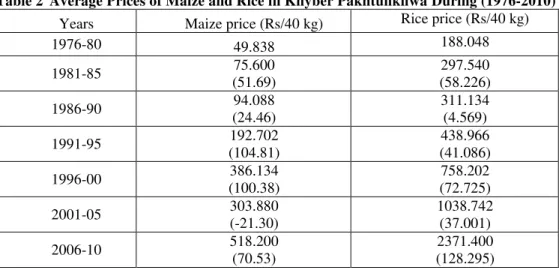
the price of maize from years 1976-80 till 1996-00.Than there is a decrease of 21.30% during the years 1996-00 to 2001-05. 2006-10 shows the highest increase of 70.53% in maize price. However the prices of rice show a consistent increasing pattern from 1976-80 to 2006-10.3.1.1 Non-price Factors (area, yield and rainfall)
Table 2 shows the total area, production and yield (5-years averages) of maize in Khyber Pakhtunkhwa from the period 1976-80 to 2006-10. Area under cultivation is an indirect measure of productivity. There is an increase of 25.24% in the area (408.4 ha) under maize crop during the years 1976-80 to 1981-1985. The slight increase trend continues till 1996-00. Average of years 2001-05 and 2006-10 shows a decrease of 3.05% and 5.39% as the area under maize was reduced to 517.6 ha and 489.7 ha respectively. In 1976-80 the average production and yield was 407.9 thousand tons and 1251.5 kg per hectares respectively. While in 2006-10 the average total production and yield was 863.0 thousand tons and 1761.7 kg per hectares respectively which shows that there is 111.57% and 40.76% increase in total production and yield. The highest average total production (875.0 thousand tons) was recorded in the years 2000-05, while the highest average yield (1761.7 kg per hectare) was recorded the years 2006-2010.
Table 2 Average Prices of Maize and Rice in Khyber Pakhtunkhwa During (1976-2010)
Years Maize price (Rs/40 kg) Rice price (Rs/40 kg)
1976-80 49.838 188.048
1981-85 75.600
(51.69)
297.540 (58.226)
1986-90 94.088
(24.46)
311.134 (4.569)
1991-95 192.702
(104.81)
438.966 (41.086)
1996-00 386.134
(100.38)
758.202 (72.725)
2001-05 303.880
(-21.30)
1038.742 (37.001)
2006-10 518.200
(70.53)
2371.400 (128.295) Source: GoP, 2010-2011.
Note: Figures in parenthesis shows percentage change (referrence year is 1976-80 for both crops).
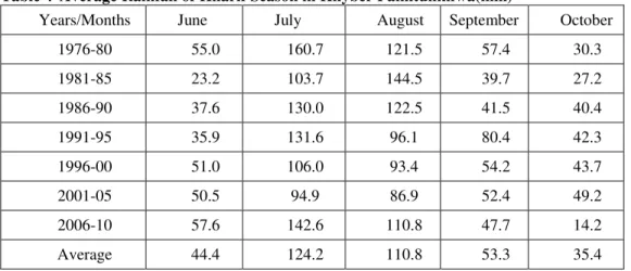
Table 3 shows the 5-years average rainfall of kharif season in Khyber Pakhtunkhwa. The average rainfall in the month of June is 44.4 mm. The highest average rainfall 57.6 mm was recorded during the years 2006-10, while the minimum average rainfall was recorded 23.2 mm during the years 1981-85. High rainfall was recorded in the months of July as compared to June. July receives the highest average rainfall in the entire kharif season during the years 1976-80 to 2006-10 i.e. 124.2 mm. The highest average rainfall was recorded 160.7 mm during 1976-80 and the lowest was 94.9 mm during 2001-05.
40
Table 3 Average Area, Production and Yield of Maize in Khyber Pakhtunkhwa During (1976-2010)
Year Area (000) ha Production (000) tons Yield (kg/ha)
1976-80 326.1 407.9 1251.5
1981-85 408.4
(25.24)
534.2 (30.96)
1317.9 (5.30)
1986-90 473.8
(16.01)
675.8 (26.51)
1424.3 (8.08)
1991-95 519.8
(9.71)
781.2 (15.60)
1502.7 (5.50)
1996-00 533.9
(2.71)
818.2 (4.74)
1532.3 (1.97)
2001-05 517.6
(-3.05)
875.0 (6.94)
1691.0 (10.36)
2006-10 489.7
(-5.39)
863.0 (-1.37)
1761.7 (4.18) Source: GoP, 2010-2011
Note: Figures in parenthesis shows percentage change.
The average rainfall further decreased in the month of September and is 53.3 mm during the years 1976-80 to 2006-10. Where the highest average rainfall was recorded 80.4 mm during 1991-95 and the lowest was 39.7 mm during 1981-85.
Table 4 Average Rainfall of Kharif Season in Khyber Pakhtunkhwa(mm)
Years/Months June July August September October
1976-80 55.0 160.7 121.5 57.4 30.3
1981-85 23.2 103.7 144.5 39.7 27.2
1986-90 37.6 130.0 122.5 41.5 40.4
1991-95 35.9 131.6 96.1 80.4 42.3
1996-00 51.0 106.0 93.4 54.2 43.7
2001-05 50.5 94.9 86.9 52.4 49.2
2006-10 57.6 142.6 110.8 47.7 14.2
Average 44.4 124.2 110.8 53.3 35.4
Source: Pakistan Metrological Department (Peshawar).
October receives the lowest average rainfall in the entire kharif season during the years 1976-80 to 2006-10 i.e. 35.4 mm, where the highest average rainfall was recorded 49.2 mm during the years 2001-05 while the lowest was 14.2 mm during 2006-10.
3.2 Model Adequacy Tests
41
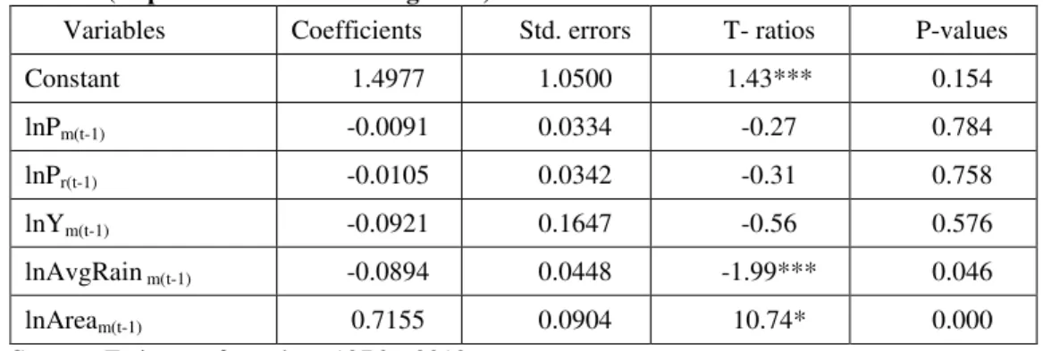
3.3 Estimates of Acreage Response of MaizeTable 5 shows the vector auto regression analysis at one lag. The model estimated contains natural log of area as explained variable with natural log of lag maize price, natural log of lag rice price, natural log of lag maize yield, natural log of lag average rainfall and natural log of lag area as explanatory variables with one year. The negative coefficient of lagged maize price (-0.0091) in the acreage equation bears insignificant relationship with maize acreage, and indicates that price do not influence area under cultivation. Result is similar to that of Gulati and Kelley (1999) who observed that the price factor is not a significant variable explaining area changes. However, it opposes the finding of Mahmood et al. (2007), Molua (2010) and Bailey and Womack (1985). The estimate for lag rice price i.e. -0.0105 has proper sign but statistically insignificant. It indicates that there is no significant effect of rice price on maize area response. This result contradicts the observation of Molua (2010), that acreage of rice in Cameroon is influenced by competitive crop, maize price but shows similarity to the observation of Bailey and Womack (1985), in certain regions of United States where major competing crops were found to have insignificant affect on wheat acreage. The lag yield estimate -0.0921 is insignificant with improper sign. Result suggests no significant effect of lag yield on maize growers’ behavior as like Mahmood et al. (2007). These results are in contrast to the findings of Tey et al. (2009) and Molua (2010), which shows significant effect of lag yield on rice area allotment in Malaysia and Cameroon, respectively. The estimated coefficient for lag rainfall (0.0894) is relatively significant, with expected sign. The significant negative coefficient of lagged rainfall indicates that last year rainfall affected the current year acreage allotment with an inverse relationship. If previous year rainfall goes up by 1 cent, mean current year acreage will go down by 0.0894 cent. This result is in conformity with the results of leaver (2004) for tobacco crop. The result is in contradiction with the findings of Molua (2010) who observed significant positive relation between last year rainfall and present year rice area allocation decision. The coefficient of the lagged dependent (0.7155) is statistically significant at 1% level with positive sign. This implies that if lag area is increased by 1 cent it will lead, on average, to an increase of about 0.7155 cent in current acreage. This tends to confirm the hypothesis of Nerlove's partial adjustment model; farmers do not adjust their acreage planted instantaneously to changes in prices and technology. Rather, they adjust to the optimum acreage level over time.
Table 5 Estimates of the Acreage Response of Maize in Khyber Pakhtunkhwa (Dependent Variable = Log Area)
Variables Coefficients Std. errors T- ratios P-values
Constant 1.4977 1.0500 1.43*** 0.154
lnPm(t-1) -0.0091 0.0334 -0.27 0.784
lnPr(t-1) -0.0105 0.0342 -0.31 0.758
lnYm(t-1) -0.0921 0.1647 -0.56 0.576
lnAvgRain m(t-1) -0.0894 0.0448 -1.99*** 0.046
lnAream(t-1) 0.7155 0.0904 10.74* 0.000
Source: Estimates from data, 1976 – 2010.
42
The value of R2 is 0.927 which is quite high and shows that the variables included in the function account for more than 90 % of the variation in maize area during the period under reference. The value of P>Chi2 (0.000) shows that the model is over all good fit.
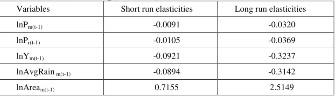
Table 6 Short and Long Run Elasticities for Area under Maize in Khyber Pakhtunkhwa During (1976-2010)
Variables Short run elasticities Long run elasticities
lnPm(t-1) -0.0091 -0.0320
lnPr(t-1) -0.0105 -0.0369
lnYm(t-1) -0.0921 -0.3237
lnAvgRain m(t-1) -0.0894 -0.3142
lnAream(t-1) 0.7155 2.5149
Source: Estimates from data, 1976 – 2010.
Table 6 shows short and long run price and non-price elasticities. For maize acreage, short run and long run market maize price elasticity is worked out as - 0.0091 and - 0.0320, while short run and long run rice price elasticity is - 0.0105 and - 0.0369, respectively but not with any significant influence. Short and long run elasticity of insignificant variable, lag maize yield is - 0.0921 and - 0.3237. In case of rainfall, response variable (area) is inelastic to the independent variable (average rainfall). In the short run, a one per cent increase in rainfall decreases total area by 0.0894 per cent and decreases 0.3142 per cent in the long run. Average rainfall shows little effect on the decision of farmers regarding allocation of land to maize. The area in long run is perfectly elastic to the lag area i.e. one per cent increase in lag area bring about 2.5149 per cent increase in area allocation to maize crop.
4. Conclusıon and Recommendatıons
43
ReferencesBailey, K. W., & Womack, A. W. (1985). Wheat Acreage Response: A Regional Econometric İnvestigation. Southern Journal of Agricultural Economics, 171-181. FAO. (2012). FAOSTAT. Food and Agricultural Organization of the United Nations.
Retrieved on 20th August, 2013.
GoP. (2011). Agricultural Statistics of Pakistan, 2010-2011. Ministry of Food and Agriculture,Economic Wing, Islamabad, Pakistan.
Gujarati, D. N., & Porter, D. C. (2003). Basic Econometrics, 5th Edition. McGraw-Hill Inc. New York, 10020.
Gulati, A., & Kelley, T. (1999). Trade Liberalization and Indian Agriculture. Oxford University Press.
Gurikar, R. Y. (2007). Supply Response of Onion in Karnataka State: An Econometric Analysis. Unpublished MS thesis submitted to the University of Agricultural Sciences, Dharwad, India. p. 62.
Haile, M. G., Kalkuhl, M., & Barun, J. V. (2013). Short-term Global Crop Acreage Response to İnternational Food Prices and İmplications of Volatility. ZEF-Discussion Papers on Development Policy No.175. p. 38.
Leaver, R. (2004). Measuring the Supply Response Function of Tobacco in Zimbabwe. Agrekon 43(1), 113-131.
Mahmood, M. A., Sheikh, A. D. & Kashif, M. (2007). Acreage Supply Response of Rice in Punjab, Pakistan. Journal of Agricultural Research 45(3), 231-236.
McKay, A., Morrissey, O. & Vaillant, C. (1999). Aggregate Agricultural Supply Response in Tanzania. Journal of International Trade and Economic Development 8(1), 107-123. Molua, E. L. (2010). Price and Non-price Determinants and Response of Rice in Cameroon.
ARPN, Journal of Agricultural and Biological Sciences 5(3), 20-25.
Mushtaq, K., & Dawson, P. J. (2002). Acreage Response in Pakistan: A Cointegration Approach. Agricultural Economics 27, 111-121.
Nerlove, M. (1958). The Dynamics of Supply: Estimation of Farmers’ Response to Price. John Hopkins Press.
Patil, K. R., Patil, B. L., Basavaraja, H., Kunnal, L. B., Sonnad, J. S. & Havaldar, Y. N. (2012). Supply Response of Arecanut in Karnataka State, Karnataka. J. Agric. Sci 25(4), 437-440.
PARC. (2013). Pakistan Agricultural Research Council. Islamabad, Pakistan.
Sangwan, S. S. (1985). Dynamics of Cropping Pattern in Haryana: A Supply Response Analysis. The Developing Economies 23(2), 173-186.
Tchereni, B. H., & Tchereni, T. H. (2013). Supply Response of Maize to Price and Non-price İncentives in Malawi. Journal of Economics and Sustainable Development 4(5), 141-152. Tey, Y. S., Darham, S., Noh, A. F. M., & Idris, N. (2009). Acreage Response of Rice: A Case
Study in Malaysia. Munich Personal RePEc Archive.
Tripathi, A. (2008). Estimation of Agricultural Supply Response Using Cointegration Approach. A report submitted under visiting research scholar programme, 2008. Indira Gandhi Institute of Development Research, Mumbai-India p. 49.