A new method for deriving glacier centerlines applied to glaciers in Alaska and northwest Canada

(1)

TCD

7, 5189–5229, 2013

A new method for deriving glacier

centerlines

C. Kienholz et al.

Title Page

Abstract Introduction

Conclusions References

Tables Figures

◭ ◮

Back Close

Full Screen / Esc

Printer-friendly Version Interactive Discussion

Discussion

P

a

per

|

D

iscussion

P

a

per

|

Discussion

P

a

per

|

Discuss

ion

P

a

per

|

The Cryosphere Discuss., 7, 5189–5229, 2013 www.the-cryosphere-discuss.net/7/5189/2013/ doi:10.5194/tcd-7-5189-2013

Open Access

The Cryosphere

Discussions

This discussion paper is/has been under review for the journal The Cryosphere (TC). Please refer to the corresponding final paper in TC if available.

A new method for deriving glacier

centerlines applied to glaciers in Alaska

and northwest Canada

C. Kienholz1, J. L. Rich1, A. A. Arendt1, and R. Hock1,2

1

Geophysical Institute, University of Alaska Fairbanks, USA

2

Department of Earth Sciences, Uppsala University, Uppsala, Sweden

Received: 6 October 2013 – Accepted: 16 October 2013 – Published: 25 October 2013 Correspondence to: C. Kienholz (christian.kienholz@gi.alaska.edu)

Published by Copernicus Publications on behalf of the European Geosciences Union.

(2)

TCD

7, 5189–5229, 2013

centerlines

C. Kienholz et al.

Title Page

Tables Figures

◭ ◮

Back Close

Full Screen / Esc

Discussion

P

a

per

|

D

iscussion

P

a

per

|

Discussion

P

a

per

|

Discuss

ion

P

a

per

Abstract

This study presents a new method to derive centerlines for the main branches and major tributaries of a set of glaciers, requiring glacier outlines and a digital elevation model (DEM) as input. The method relies on a “cost grid – least cost route approach” that comprises three main steps. First, termini and heads are identified for every glacier. 5

Second, centerlines are derived by calculating the least cost route on a previously es-tablished cost grid. Third, the centerlines are split into branches and a branch order is allocated. Application to 21 720 glaciers in Alaska and northwest Canada (Yukon, British Columbia) yields 41 860 centerlines. The algorithm performs robustly, requiring no manual adjustments for 87.8 % of the glaciers. Manual adjustments are required pri-10

marily to correct the locations of glacier heads (5.5 % corrected) and termini (3.5 % cor-rected). With corrected heads and termini, only 1.4 % of the derived centerlines need edits. A comparison of the lengths from a hydrological approach to the lengths from our longest centerlines reveals considerable variation. Although the average length ra-tio is close to unity, only ∼50 % of the 21 720 glaciers have the two lengths within 15

10 % of each other. A second comparison shows that our centerline lengths between lowest and highest glacier elevations compare well to our longest centerline lengths. For>70 % of the 4350 glaciers with two or more branches, the two lengths are within 5 % of each other. Our final product can be used for calculating glacier length, conduct-ing length change analyses, topological analyses, or flowline modelconduct-ing.

20

1 Introduction

Glacier centerlines are a crucial input for many glaciological applications. For example, centerlines are important for determining glacier length changes over time (Leclercq et al., 2012; Nuth et al., 2013), analyzing velocity fields (Heid and Kääb, 2012; Melko-nian et al., 2013), estimating glacier volumes (Li et al., 2012; Linsbauer et al., 2012), 25

(3)

TCD

7, 5189–5229, 2013

centerlines

C. Kienholz et al.

Title Page

Tables Figures

◭ ◮

Back Close

Full Screen / Esc

Discussion

P

a

per

|

D

iscussion

P

a

per

|

Discussion

P

a

per

|

Discuss

ion

P

a

per

|

Also, glacier length, derived from centerlines, is an important parameter for glacier in-ventories (Paul et al., 2009).

So far, most of the above applications have relied on labor-intensive manual digi-tization of centerlines. The few studies that derive centerlines fully automatically use a hydrological approach and/or derive only one centerline per glacier (Schiefer et al., 5

2008; Le Bris and Paul, 2013). Here, we present a new algorithm that allows for deriving multiple centerlines per glacier based on a digital elevation model (DEM) and outlines of individual glaciers. Moreover, this algorithm splits the centerlines into branches and classifies them according to a geometry order. The approach is tested on all glaciers in Alaska and adjacent Canada with an area>0.1 km2, corresponding to 21 720 out of 10

26 950 glaciers. We carry out a quality analysis by visual inspection of the centerlines, and compare the derived lengths to the lengths obtained from alternative approaches.

2 Previous work

The automatic derivation of glacier centerlines and thereof retrieved glacier length is considered challenging (Paul et al., 2009; Le Bris and Paul, 2013). Consequently, only 15

few automated approaches have been proposed so far (Schiefer et al., 2008; Le Bris and Paul, 2013) and often, centerlines have been digitized manually even for large-scale studies.

In their large-scale study, Schiefer et al. (2008) applied an automated approach to all British Columbia glaciers that is based on hydrology tools. For each glacier, this 20

approach derives one line that represents the maximum flow path that water would take over the glacier surface. Schiefer et al. (2008) find that these lengths are 10–15 % longer than distances measured along actual centerlines. Because lower glacier areas (∼ablation areas) are typically convex in cross-section, their flow paths are deflected toward the glacier margins, which leads to length measurements that are systematically 25

too long in these cases. While systematically biased lengths in a glacier inventory can be corrected for, the actual lines need major manual corrections before they can

(4)

TCD

7, 5189–5229, 2013

centerlines

C. Kienholz et al.

Title Page

Tables Figures

◭ ◮

Back Close

Full Screen / Esc

Discussion

P

a

per

|

D

iscussion

P

a

per

|

Discussion

P

a

per

|

Discuss

ion

P

a

per

be used in glaciological applications such as flowline modeling. Therefore, Paul et al. (2009) suggest the use of the above automated algorithm in the concave (i.e., higher) part of the glacier, combined with manual digitization in the convex (lower) part of the glacier.

Le Bris and Paul (2013) present an alternative method for calculating glacier cen-5

terlines based on a so-called “glacier axis” concept, which derives one centerline per glacier between the highest and the lowest glacier elevation. Le Bris and Paul (2013) first establish a line (the “axis”) between the highest and the lowest glacier point, which is then used to compute center points for the glacier branches. These center points are connected, starting from the the highest glacier elevation and following certain rules 10

(e.g., “always go downward”, “do not cross outlines”). Smoothing of the resulting curve leads to the final centerline. The algorithm is applicable to most glacier geometries, yielding results similar to manual approaches (Le Bris and Paul, 2013). A limitation of their approach is the fact that the derived centerline between the highest and lowest glacier elevation does not necessarily represent the longest glacier centerline or the 15

centerline of the main branch, either one of them often required in glaciological ap-plications. For example, for glacier inventories, it is recommended to measure glacier length along the longest centerline, or, alternatively, to average the lengths of all glacier branches (Paul et al., 2009).

3 Test site and data 20

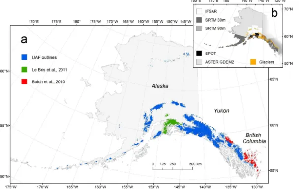
Our algorithm is tested on glaciers located in Alaska and adjacent Canada (Fig. 1a). For brevity, we hereafter refer to these glaciers as Alaska glaciers. From the complete Alaska glacier inventory (Arendt et al., 2013), we extract all glaciers with a minimal area threshold of>0.1 km2, thus eliminating small glacierets and possible perennial snowfields. This results in 21 720 glaciers with 86 400 km2of ice total, which accounts 25

(5)

TCD

7, 5189–5229, 2013

centerlines

C. Kienholz et al.

Title Page

Tables Figures

◭ ◮

Back Close

Full Screen / Esc

Discussion

P

a

per

|

D

iscussion

P

a

per

|

Discussion

P

a

per

|

Discuss

ion

P

a

per

|

The Alaska glacier inventory comprises glacier outlines derived from satellite im-agery taken between ∼2000 and 2012. The outlines used herein either stem from manual digitization at the University of Alaska Fairbanks or from automated band ratio-ing followed by visual quality checks and manual corrections (Bolch et al., 2010; Le Bris et al., 2011, Fig. 1a).

5

Four DEM products are combined to create a continuous 60 m DEM consistent with the time-span covered by the glacier outlines (Fig. 1b). South of 60◦N, we rely on the Shuttle Radar Topography Mission (SRTM) DEM (http://www2.jpl.nasa.gov/srtm, ac-cess: 25 July 2013), taken in February 2000 (Farr et al., 2007). Over Alaska, the SRTM DEM has a native spatial resolution of 30 m, while the resolution is 90 m over Canada. 10

North of 60◦N, we use a high quality DEM derived from airborne Interferometric Syn-thetic Aperture Radar (IFSAR) data obtained in 2010 (Geographic Information Network of Alaska GINA, http://ifsar.gina.alaska.edu, access: 25 July 2013). For areas not cov-ered by the IFSAR DEM, we use DEMs derived from data from the High Resolution Stereo (HRS) imaging instrument onboard the Système Pour l’Observation de la Terre 15

(SPOT) satellite taken within the scope of the SPIRIT program (time span 2007–2008, Korona et al., 2009) and the Advanced Spaceborne Thermal Emission and Reflection Radiometer (ASTER) instrument onboard the Terra satellite (ASTER GDEM2, time span 2000–2011, Tachikawa et al., 2011, http://asterweb.jpl.nasa.gov/gdem, access: 25 July 2013). The individual DEM tiles are merged into one dataset giving priority 20

to the highest quality DEM available for each area. While the used DEMs represent roughly the same time span, the goals and scopes of the individual campaigns are dif-ferent, which becomes apparent in the contrasting quality of the DEMs. For example, the GDEM has nearly global coverage, but limited quality, while the IFSAR DEM is of high quality, but only available for parts of Alaska.

25

(6)

TCD

7, 5189–5229, 2013

centerlines

C. Kienholz et al.

Title Page

Tables Figures

◭ ◮

Back Close

Full Screen / Esc

Discussion

P

a

per

|

D

iscussion

P

a

per

|

Discussion

P

a

per

|

Discuss

ion

P

a

per

4 Method

Our goal is to design an algorithm that (1) creates centerlines for the main glacier branches as well as major tributaries, (2) yields a quality comparable to a manual ap-proach, and (3) requires minimal data and manual intervention. It would be desirable to derive centerlines that represent actual flowlines (i.e., ice trajectories), however, this 5

would require coherent velocity fields without gaps. While corresponding algorithms are applied for single glaciers (e.g., McNabb et al., 2012), stringent velocity data require-ments make large-scale applications diffi_{cult. Here, we aim at obtaining centerlines} that are close to flowlines by only using glacier outlines and a DEM as input. Such cen-terlines diff_{er from flowlines mostly in areas, where centerlines from di}ff_{erent glacier} 10

branches converge. Actual flowlines would not converge completely, but run roughly in parallel to the glacier terminus, as illustrated, for example, by Farinotti et al. (2009). Although not entirely consistent with real flowlines, centerlines are used for modeling purposes (e.g., Oerlemans, 1997b; Leclercq et al., 2012). They can also be used for applications that generally have lower requirements than does modeling (e.g., deter-15

mining length changes, deriving glacier length for inventories).

Here, we apply a method that we call a “cost grid – least cost route approach”. The workflow consists of three main steps that are implemented using the PythonTM pro-gramming language and ESRI®’s arcpy module. The first step comprises the identifi-cation of glacier termini and glacier heads. The second step encompasses the calcula-20

tion of a cost grid, followed by determining and optimizing the least cost route to derive the glacier centerlines. In the third step, these centerlines are split into branches and a geometry order is introduced. Because the three steps are associated with diﬀ_erent uncertainties, we have separate modules for each step of the algorithm.

4.1 Step 1 – identification of glacier heads and termini 25

(7)

TCD

7, 5189–5229, 2013

centerlines

C. Kienholz et al.

Title Page

Tables Figures

◭ ◮

Back Close

Full Screen / Esc

Discussion

P

a

per

|

D

iscussion

P

a

per

|

Discussion

P

a

per

|

Discuss

ion

P

a

per

|

and one head for each major glacier branch. The centerlines eventually run from each glacier head to the terminus.

4.1.1 Glacier terminus

A natural way of identifying the glacier terminus is by extracting the lowest glacier cell (e.g., Le Bris and Paul, 2013). To better constrain our lowest point to the actual termi-5

nus, we apply the corresponding query on a low-pass filtered and “filled” DEM. “Filling” refers to removing depressions within the DEM that could hamper the identification of the actual glacier terminus. We consider filling and filtering as most important for large receding glaciers, ending in flat terrain, that are generally characterized by a rough surface with numerous depressions.

10

Figure 2a shows the glacier terminus as automatically obtained for Gilkey Glacier, an outlet glacier of the Juneau Icefield located in southeast Alaska.

4.1.2 Glacier heads

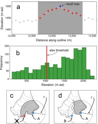
Since we aim to derive centerlines of all major glacier branches, we need to identify heads for each of these branches. A three-step procedure is adopted to identify these 15

heads (Fig. 3). First we identify local elevation maxima along the glacier outlines. Our algorithm samples the DEM in predefined steps (100 m) along the glacier outline (in-cluding nunataks) and then compares each sampled elevation to its neighboring points along the outline. A possible glacier head is identified if the local point is higher than its neighbors (five neighbors in each direction, Fig. 3a) and if the point is higher than 20

the lowest one third of the elevation distribution of all the sampled points of the cor-responding glacier (Fig. 3b). We apply the second criterion since glacier heads are typically located at higher elevations. We also want to avoid assigning centerlines to low-lying minor tributaries.

Given the irregular shapes of typical glacier outlines, the workflow above can result in 25

multiple heads per glacier branch. To remove multiple heads per branch, we introduce

(8)

TCD

7, 5189–5229, 2013

centerlines

C. Kienholz et al.

Title Page

Tables Figures

◭ ◮

Back Close

Full Screen / Esc

Discussion

P

a

per

|

D

iscussion

P

a

per

|

Discussion

P

a

per

|

Discuss

ion

P

a

per

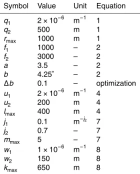
a minimum linear distancer (m) that the derived heads must be apart. Since larger glaciers tend to have wider basins, we define r as a function of glacier area S (m2) according to Eq. 1:

r= (

q1·S+q2 : r ≤rmax rmax : r >rmax

(1)

q₁,q₂andr_maxare constants given in Table 1. In case one or more heads are withinr, 5

we only retain the highest head and erase all others (Fig. 3c). If two heads are apart by a distance less thanr but separated by a nunatak, both heads are retained. A nunatak is identified if the circle defined byr splits the glacierized area into two or more parts (Fig. 3d).

In case no head is identified using the above steps, which can be the case for small 10

glaciers, we identify the highest glacier elevation as the glacier head. In case of Gilkey Glacier, 77 heads are identified (Fig. 2a).

4.2 Step 2 – establishment of cost grid and determination of least cost route

This step establishes a cost or penalty grid (here used as synonyms) with high values at the glacier edge and in upper reaches of the glacier. The penalty values decrease 15

towards the glacier center as well as towards lower elevations. The least cost route from a glacier head to the glacier terminus yields the centerline.

4.2.1 Cost/penalty grid and route cost

First, we create a penalty grid with 10 m×10 m cell size according to Eq. 2. We choose

this small cell size to obtain a detailed representation of the glacier outlines in the 20

(9)

TCD

7, 5189–5229, 2013

centerlines

C. Kienholz et al.

Title Page

Tables Figures

◭ ◮

Back Close

Full Screen / Esc

Discussion

P

a

per

|

D

iscussion

P

a

per

|

Discussion

P

a

per

|

Discuss

ion

P

a

per

|

glacier is computed by

pi=

_max(_d₎₋_d

i

max(d) ·f1 a

+

_z

i−min(z)

max(z)−min(z)·f2

b

(2)

d_i is the Euclidean distance from celli to the closest glacier edge and z_i is the corre-sponding elevation. max(d), max(z) and min(z) are the glacier’s maximum Euclidean distance, maximum elevation, and minimum elevation, respectively. The “stretching” 5

factorsf₁andf₂and the “weighting” exponentsaandbobtained for our study area are given in Table 1.

The first term max(d)−di

max(d) normalizesdi to the maximum Euclidean distance found on

the glacier, and leads to a Euclidean penalty contribution that ranges between zero and one (i.e., zero at the cell(s) with max(d) and one along the glacier edge). By multiplying 10

the term with f1, we stretch the normalized values to a range between zero and f1. The second term zi−min(z)

max(z)−min(z) normalizes the elevation of each grid cell to the elevation range of the entire glacier, and yields an elevation penalty contribution that is zero at the glacier terminus, where z=_min(_z_{), and one at the highest glacier point, where} z=_max(_z_). _f₂ _{stretches these values to a range between zero and} _f₂_{. While the first} 15

term tends to force the least-cost route to the glacier center, the second term tends to force it downslope. The exponentsaand b control the weight each of these terms have. The normalization in Eq. 2 is implemented to make the sameaandbexponents better transferable to glaciers of diﬀ_{erent size and geometry.}

f₁andf₂stretch the normalized values back to actual glacier dimensions. Both factors 20

are derived from medium sized glaciers located in the Alaska Range that were used to calibrate the initialaandbexponents. As we applied an unnormalized version of Eq. 2 to calibrateaandb, that is,p_i=_(max(_d₎₋_d

i)) a₊

(z_i−min(z))b,f₁(1000, ∼equivalent

to max(d)calib.) andf2(3000,∼equivalent to max(z)calib.−min(z)calib.) are necessary to use these initially calibratedaandbvalues in the normalized Eq. (2).

25

To obtain plausible centerlines, a strong increase in the penalty values is required close to the glacier boundary and at higher glacier elevations. High Euclidean

(10)

TCD

7, 5189–5229, 2013

centerlines

C. Kienholz et al.

Title Page

Tables Figures

◭ ◮

Back Close

Full Screen / Esc

Discussion

P

a

per

|

D

iscussion

P

a

per

|

Discussion

P

a

per

|

Discuss

ion

P

a

per

induced penalty values at the glacier boundary are crucial to prevent centerlines from reaching too close to the glacier edge, which would not match the expected course of flowlines. A strong elevation-induced penalty gradient at higher glacier altitudes is important to ensure that centerlines choose the correct branch from the start. By using a and b as exponentials and not as coeﬃ_{cients, we do obtain the highest penalty} 5

gradients close to the glacier edges and at high glacier elevations.

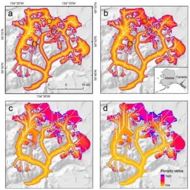
Figure 4a shows the initial cost grid obtained for Gilkey Glacier. The first part of Eq. (2) is dominating (penalties decrease strongly towards the branch centers), while the second part of the equation has a lower eﬀ_ect.

Using the cost grid obtained from Eq. (2), we calculate the least cost route from 10

each head to the glacier terminus, which corresponds to the path with the minimum route cost. The route costcis defined by the sum of the penalty valuespi between the

glacier head and the terminus,

c=

I

X

i=1

pi (3)

whereI is the total number of cells crossed from the glacier head to the glacier ter-15

minus. The optimal path is not necessarily the shortest path (minimalI), because the penalty valuesp_i are not constant. For example, given a meandering glacier, the short-est route is expensive, because it crosses cells with very high penalty values at the edge of the glacier. Instead, it is cheapest to stay near the center of the glacier. Al-though this route crosses more cells (higherI), the resulting sum of penalties is smaller 20

as the penalty values (pi) are considerably smaller near the glacier center.

In a next step, we convert the above least cost route, which is obtained as a raster dataset, to a vector format. We then smooth the corresponding curve using a standard Polynomial Approximation with Exponential Kernel (PEAK) algorithm. This algorithm calculates a smoothed centerline by applying a weighted average on the vertices of 25

(11)

TCD

7, 5189–5229, 2013

centerlines

C. Kienholz et al.

Title Page

Tables Figures

◭ ◮

Back Close

Full Screen / Esc

Discussion

P

a

per

|

D

iscussion

P

a

per

|

Discussion

P

a

per

|

Discuss

ion

P

a

per

|

the length of the subsegment,l(m), for every glacier individually, by

l= (

u₁·S+u₂ : l≤l_max

l_max : l>l_max (4)

whereSis the glacier area in m2. The constantsu1,u2andlmaxare given in Table 1.l is increased as a function of the glacier area to account for the wider branches and the smooth course of the centerline typical for larger glaciers.

5

For simple glacier geometries, the first term alone in Eq. (2) already creates plau-sible centerlines; however, for more complex geometries, the resulting centerlines can “flow” unreasonably upslope and choose a wrong route. Because elevation (or slope) is neglected in the first term, the centerlines stick to the glacier center regardless of the topography. To remedy this problem, the elevation-dependent term is essential in 10

Eq. (2). The elevation-dependent term also forms the basis for the optimization step introduced next.

4.2.2 Optimization

During the optimization we aim to find a combination ofa and b values (Eq. 2) that provides the most plausible solution for each centerline. Our approach is based on the 15

following considerations: if a narrow and a wide basin are connected in their upper reaches, centerlines will typically flow through the wide basin, because the penalty val-ues are smaller in the center of the wide basin compared to the center of the narrow basin. This is illustrated in Fig. 4a, where wide basins have lower penalty values in the center than narrow basins. In some cases, the centerlines may flow a significant 20

distance upslope and make a major detour to reach a wider basin, and still have min-imum route cost. In these cases, the low penalty values in the center of the reached wide basin overcompensate for the additional penalties due to the detour. This implies that the weight of the second term of Eq. (2) is too low compared to the weight of the first term. Incrementally increasing the second part of Eq. (2) will eventually force the 25

(12)

TCD

7, 5189–5229, 2013

centerlines

C. Kienholz et al.

Title Page

Tables Figures

◭ ◮

Back Close

Full Screen / Esc

Discussion

P

a

per

|

D

iscussion

P

a

per

|

Discussion

P

a

per

|

Discuss

ion

P

a

per

centerline to take a route that is shorter and typically characterized by less upslope flow. Ideally, this is the correct centerline.

To obtain the initial centerlines, we apply a and b values of 4.25 and 3.5, respec-tively (Table 1), as derived from tests in the Alaska Range. During the optimization, we keepa constant and raise b in discrete steps∆_b _{(0.1 per iteration, Table 1), thereby} 5

increasing the weight of the elevation component in Eq. (2). Not all centerlines require an optimization, and in case centerlines require optimization,b can not be increased infinitely, as this leads to a loss of the expected “natural” course of the centerline. Fig-ure 4a illustrates this on Gilkey Glacier, where most initial centerlines have plausible routes. Only the centerlines marked by circles have implausible routes with major up-10

slope flow and thus clearly need optimization. Figure 4b–d shows that an increase of b improves the lines in need of optimization (i.e., the implausible centerlines circled in Fig. 4a take the correct route in Fig. 4b), while it may diminish the quality of the remaining centerlines due to the higher weight of the elevation term, which forces cen-terlines to “cut corners” instead of sticking to the glacier center. Accordingly, a criterion 15

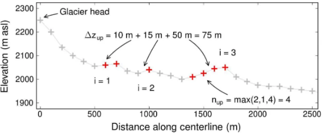
is needed to determine whether optimization is necessary, and in case it is, to decide when to terminate the optimization. For this purpose, we sample the DEM along each centerline and determine the total elevation increase in m (∆_z

up, Eq. (5), Fig. 5) and the maximum number of samples with continuously increasing elevation (nup, Eq. (6), Fig. 5).

20

∆_z_up=

I

X

i=1

∆_z_up,_i ₍₅₎

nup=max(nup,i) (6)

Iis the total number of individual centerline sections with upslope flow.

∆_z_up _and_n_up _{are used to calculate the iteration threshold}_m_{(Eq. 7). Comparison of} 25

(13)

TCD

7, 5189–5229, 2013

centerlines

C. Kienholz et al.

Title Page

Tables Figures

◭ ◮

Back Close

Full Screen / Esc

Discussion

P

a

per

|

D

iscussion

P

a

per

|

Discussion

P

a

per

|

Discuss

ion

P

a

per

|

carried out.

m= (

n_up+_j 1·∆z

j₂

up : m≤mmax m_max : m>m_max

(7)

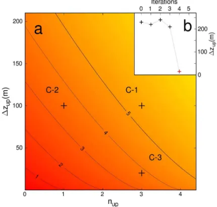
j1,j2andmmaxare given in Table 1. Equation (7) mimicks our concept of having a high number of iterations if a largenup coincides with a high∆zup(“worst case”, e.g., C-1 in Fig. 6a), as this is a very strong indicator for a wrong course of the preliminary center-5

line. If bothnup and ∆zup are zero,mis also zero as we assume that the preliminary centerline already takes the correct branch. If a high∆_z_up _{occurs in conjunction with} a lowern_up or vice versa (e.g., C-2 and C-3 in Fig. 6a),mis reduced compared to the worst case scenario. In those cases, we are less confident that the lines are actually wrong as such patterns occur occasionally even if the line takes the correct branch. 10

For example, a 2-like pattern can be caused by blunders in the DEM, while a C-3-like pattern can occur along the centerlines of larger glaciers. By using Eq. (7) we allocate fewer iterations to these possibly correct cases than to cases where we are more certain that they are actually wrong (C-1).

Tests indicate that many wrong centerlines shift to the correct branch within less than 15

five iterations. Thus, we limit the maximum number of iterationsmmaxto five, no matter the magnitude ofn_up and∆_z

up. Not obtaining a better solution after five iterations may indicate wrong divides (i.e., glaciers are not split correctly, and the centerline has to flow over a divide) or problems with the DEM (i.e., blunders within a large area that can not be bypassed). A narrow branch located next to a very wide branch may also 20

prevent a correct solution within five iterations. However, even if the algorithm found the correct branch after more than five iterations, the resulting line likely had an implausible shape due to the highb value (Fig. 4d).

Figure 6b shows a typical example of the progression of∆_z_up_{during the optimization} procedure, in case there is a better branch option:∆_z_up _{remains high during the first} 25

three iterations because the centerline keeps taking the wrong branch. In iteration four, the centerline shifts to the correct branch and∆_z_up _{decreases significantly. This drop}

(14)

TCD

7, 5189–5229, 2013

centerlines

C. Kienholz et al.

Title Page

Tables Figures

◭ ◮

Back Close

Full Screen / Esc

Discussion

P

a

per

|

D

iscussion

P

a

per

|

Discussion

P

a

per

|

Discuss

ion

P

a

per

in∆_z

upis typically associated with a drop innup(not shown in Fig. 6b), which results in a lowermaccording to Fig. 6a. In most cases, the number of accomplished iterations is higher than the newm, and therefore, the optimization terminates as soon as the centerline shifts to the correct branch.

To obtain∆_z_up _and_n_up_{, we sample the DEM only along the uppermost 25 % of the} 5

centerlines’ length. Centerlines most often take the wrong route (i.e., flow upslope) in this uppermost glacier section, where the diﬀ_{erent glacier branches tend to be} inter-connected. The same is very unlikely in the lowermost glacier part, as there is typically only one branch left. Even if more than one branch is left, these branches are generally separated by nunataks that can not be crossed by centerlines. Moreover, upslope flow 10

in the uppermost glacier part is clearer evidence of a wrong route than upslope flow in lower parts, where the surface may be more irregular, for example, due to varying debris coverage. Including lower glacier parts could lead to large∆_z_up _and_n_up _values although the centerline takes the correct route.

Following the optimization, the best solution is selected from the calculated center-15

lines. We choose the solution that has the smallestnup. If two or more solutions have the samen_up, we order them according to∆_z

up and choose the one with the smallest ∆_z_up_{. If this does not lead to a unique solution either, we take the one solution with the} lowest iteration number. Selection of the best solutions yields the final set of glacier centerlines.

20

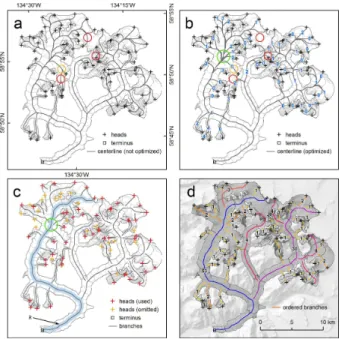
Figure 7a (corresponding to Fig. 4a) shows the preliminary set of centerlines as derived for Gilkey Glacier, while Fig. 7b shows the optimized set of glacier centerlines. The three red circles indicate implausible centerlines with significant upslope flow that are successfully adapted during the optimization step. The orange circle shows an implausible centerline that is not improved because there is no upslope flow in this 25

case (the optimization does not respond because∆_z

(15)

TCD

7, 5189–5229, 2013

centerlines

C. Kienholz et al.

Title Page

Tables Figures

◭ ◮

Back Close

Full Screen / Esc

Discussion

P

a

per

|

D

iscussion

P

a

per

|

Discussion

P

a

per

|

Discuss

ion

P

a

per

|

The derived centerlines reach all the way from the glacier heads to the glacier ter-mini. If two or more branches converge, lines start to overlap. As the optimization step can result in diﬀ_erent _b _{values for each individual centerline, the derived centerlines} do not necessarily overlap perfectly. The green circle in Fig. 7b shows an example of imperfect overlap in case of Gilkey Glacier.

5

4.3 Step 3 – Derivation of branches and branch order

The ultimate goal of this step is to remove the overlapping sections of the centerlines and to arrive at individual branches that are classified according to a geometric order. We keep the longest centerline that reaches from the head to the terminus. The re-maining centerlines are trimmed so that they reach from their head to the next larger 10

branch. If a trimmed centerline falls below a length threshold, it is deleted.

4.3.1 Branches

We consider the longest centerline as the main branch, following previous studies (Bahr and Peckham, 1996; Paul et al., 2009). This main branch is exported into a separate file. Then, from the initial file, we remove the main branch including line segments 15

within a distancek (m) of the main branch (Fig. 7c). We apply this minimum distancek because diﬀ_erent_b_{values, employed during the optimization step, can yield centerlines} that do not overlap perfectly. Centerlines may run in parallel in the same branch before they converge, or they may diverge again, after having converged higher on the glacier. k, defined according to Eq. (8), allows for eliminating such cases of imperfect overlap. 20

k= (

w₁·S+_w₂ _: _k≤k_max

k_max : k>k_max (8)

The constantsw1,w2andkmaxare given in Table 1. Larger glaciers tend to have wider branches and parallel running centerlines in the same branch may be farther apart. To

(16)

TCD

7, 5189–5229, 2013

centerlines

C. Kienholz et al.

Title Page

Tables Figures

◭ ◮

Back Close

Full Screen / Esc

Discussion

P

a

per

|

D

iscussion

P

a

per

|

Discussion

P

a

per

|

Discuss

ion

P

a

per

account for this, we increasek as a function ofS.k is not the actual branch width, but rather a minimum distance that is required to eliminate cases of imperfect overlap.

The application ofk may yield lines that are split into multiple parts (one segment from the head to the first conversion point, the second segment from the first to the second conversion point, etc.). As the segment from the first conversion point to the 5

terminus is already covered by the main branch, we keep only the one segment in contact with the glacier head and remove all the other segments.

The step above is applied iteratively to the longest centerline of the updated initial file until the number of remaining centerlines reaches either zero or their length falls below a certain length. As a length threshold, we reapplyr defined in Eq. (1). In cases 10

wherer would remove all centerlines (which may occur for small glaciers), Eq. (1) is not applied. Instead,r adopts the length of the longest centerline.

Merging of the identified individual branches yields the final set of branches. In case of Gilkey Glacier, 53 branches are obtained; 24 out of 77 lines are omitted because their length is belowr. In Fig. 7c, the heads of omitted branches are marked in orange. 15

The green circle in Fig. 7c shows an area of initially imperfect overlap after employment of step 3.

4.3.2 Branch order

The above step yields a set of branches for every glacier and also establishes a branch order using the branch length as a criterion: while the longest branch is the main 20

branch (highest-order), the shortest branch is the lowest-order branch. Next, we evalu-ate the number of side branches that contribute to each individual branch. In this case, the branch order increases with the number of contributing branches. This results in main branches that have the highest numbers allocated. The numbers decrease as the branches fork into smaller branches. “1” stands for the lowest-order branch, meaning 25

(17)

TCD

7, 5189–5229, 2013

centerlines

C. Kienholz et al.

Title Page

Tables Figures

◭ ◮

Back Close

Full Screen / Esc

Discussion

P

a

per

|

D

iscussion

P

a

per

|

Discussion

P

a

per

|

Discuss

ion

P

a

per

|

The implementation consists of a proximity analysis that is iteratively applied to each individual branch. We start by allocating an order of one (lowest-order) to every branch. Next, we iterate through the branches in the order of increasing length and flag the branches that are within a distance ofk (Eq. 8) from the one branch selected at that iteration step (the reference branch). The proximity analysis is applied only within the 5

glacierized terrain, that is, a branch separted by nunataks is not flagged unlessk is de-ceeded at a point without nunatak between branch and reference branch. By summing the individual orders of the flagged branches, we arrive at the true order of the selected reference branch. This true order is updated instantaneously because its updated value is required for the next iterations.

10

Figure 7d shows the result for Gilkey Glacier. The “53” of the main branch indicates that 53 first-order branches converge to make up the main branch.

4.4 Quality analysis and manual adjustments

The quality analysis consists of a visual check, conducted throughout the domain by evaluating the derived centerlines in conjunction with contours (50 m contour spacing), 15

shaded relief DEMs, and satellite imagery (mostly Landsat). A 25 km×25 km grid, cov-ering the entire study area, is used for guidance and keeping track of checked regions. We assess whether heads and termini are located correctly. For the termini, this means approximately at the center of the tongue; for the heads, at the beginning of a branch. The actual centerlines should flow roughly orthogonal to contour lines and parallel to 20

visible moraines.

Glacier termini are moved to the center of the tongues, and glacier heads are added, deleted or moved as needed. To determine the number of moved termini, we compare the coordinates of the initial, automatically derived termini to the coordinates of the checked termini and sum the number of cases with changed coordinates. A similar 25

analysis allows us to distinguish and quantify the two categories “added” and “deleted” heads.

(18)

TCD

7, 5189–5229, 2013

centerlines

C. Kienholz et al.

Title Page

Tables Figures

◭ ◮

Back Close

Full Screen / Esc

Discussion

P

a

per

|

D

iscussion

P

a

per

|

Discussion

P

a

per

|

Discuss

ion

P

a

per

Instead of editing the actual centerlines manually, we establish a new set of lines that we call “breaklines”. The idea is to treat these breaklines like nunataks upon rerun-ning of step 2 of our workflow. This implies that centerlines may not cross breaklines; moreover, breaklines change the derived penalty raster. Such an approach allows for eﬃ_{cient correction of wrong centerlines. For example, it is useful to adapt a centerline} 5

that did not shift into the correct branch despite the optimization procedure. A simple breakline that blocks access to the wrong branch is suﬃ_{cient to reroute the wrong} cen-terline, which is much faster than manually editing the actual centerline. In the context of the quality analysis, counting the number of set breaklines allows for quantifying wrong centerlines.

10

To obtain the final set of centerlines, steps 2 and 3 of the workflow are repeated using the adapted heads, termini and breaklines as input, without changing any of the remaining input data or parameters. To allow breaklines as an additional input, an adapted version of the code of step 2 is run.

4.5 Comparison to alternative methods 15

To identify diﬀ_{erences between alternative methods, it would be ideal to compare the} actual centerline shapes. However, quantitatively assessing shape agreement is chal-lenging, especially for a large number of glaciers. Here, we use the length as a proxy for agreement and carry out two comparisons. First, we compare the glacier lengths derived from a hydrological approach to the lengths derived from our longest center-20

lines. To obtain the hydrological lengths, we run the tool “Flow Length” from the ESRI® ArcGIS software package, which is similar to the tool applied by Schiefer et al. (2008). While this tool yields a length parameter for every glacier, it does not output an actual line that can be checked visually.

In the second comparison, we evaluate agreement between our longest centerlines 25

(19)

TCD

7, 5189–5229, 2013

centerlines

C. Kienholz et al.

Title Page

Tables Figures

◭ ◮

Back Close

Full Screen / Esc

Discussion

P

a

per

|

D

iscussion

P

a

per

|

Discussion

P

a

per

|

Discuss

ion

P

a

per

|

2013), rather than an algorithm that considers multiple heads. Unlike in the first exper-iment, we do not compare two approaches that are fundamentally diﬀ_{erent, but rather} the same approach with one diﬀ_{erent assumption regarding glacier heads. Thus, we} expect better agreement in the second experiment.

5 Results 5

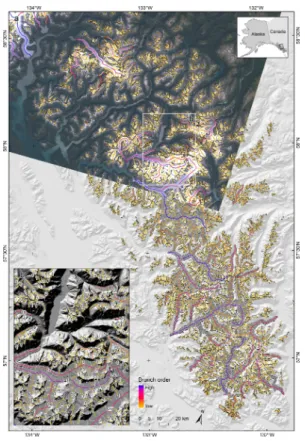
For the 21 720 glaciers with an area>0.1 km2, we obtain 41 860 centerlines, of which 8480 have a non-zero optimized iterative solution. The centerlines range in length be-tween 0.1 and 195.7 km; the summed length is 87 460 km. Mean glacier length of our sample, as derived from the respective longest centerlines, is 2.0 km. 4350 glaciers have more than one branch and the corresponding branch orders reach up to 340. 10

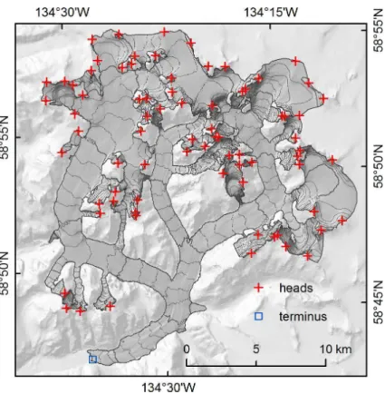
Figure 8 shows the centerlines derived for the Stikine Icefield area, located in the Coast Mountains of southeast Alaska/northwest Canada. The glacier geometries range from large outlet glaciers to medium-sized valley and small cirque glaciers.

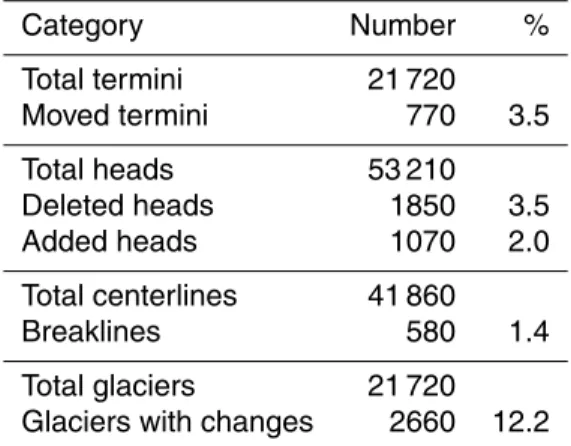
Table 2 gives an overview of the manual changes conducted during the quality analysis. 19 060 of the 21 720 glaciers (87.8 %) require no manual intervention at all. 15

2660 glaciers (12.2 %) need any kind of manual intervention within the three-step pro-cedure. Most cases of manual intervention are required to adapt the automatically derived glacier heads (1850 deleted, 1070 added) and termini (770 moved), indicating that steps 1 or 3 do not yield the expected outcome in these instances. 580 breaklines are used to adjust the course of the actual centerlines, indicating that in these cases, 20

step 2 does not yield the intended result.

(20)

TCD

7, 5189–5229, 2013

centerlines

C. Kienholz et al.

Title Page

Tables Figures

◭ ◮

Back Close

Full Screen / Esc

Discussion

P

a

per

|

D

iscussion

P

a

per

|

Discussion

P

a

per

|

Discuss

ion

P

a

per

6 Discussion

6.1 Algorithm

Despite its empirical nature, our approach yields plausible results for a wide range of glacier sizes and shapes, provided both good quality DEMs and glacier outlines are available. However, the algorithm has limitations, as shown by the quality analysis. 5

The main challenge is to automatically derive glacier heads and termini, due to the large natural variability inherent in the glacier sample with respect to size, shape and hypsometry. The actual derivation of the centerlines is less error-prone.

6.1.1 Termini

We use the lowest glacier points to automatically identify glacier termini, which can 10

lead to problems described in Le Bris and Paul (2013). Especially if glacier tongues reach low-slope terrain, which is typical for expanded-foot and piedmont glaciers, the lowest glacier cell may not be located in the center of the glacier tongue, but rather along the side of the glacier. This “pulls” the line away from the glacier center and leads to centerlines that are not realistic. Although this inconsistency only aﬀ_{ects the} 15

immediate tongue area, it may interfere with certain applications and thus requires a manual shift of the terminus. In our study area, shifting of misplaced termini accounts for a considerable number of cases requiring manual input (Table 2). Currently, we do not have a reliable automatic approach to detect and adapt such misclassified termini. In many glacierized areas, there are glaciers that drain into multiple tongues. Our al-20

gorithm identifies the lowest point as the only terminus and therefore does not account for multiple termini. To address this problem, we have to manually split these glaciers into separate catchments (i.e., one catchment per tongue), followed by treating the catchments like separate glaciers. In Alaska and northwest Canada, only a handful of glaciers drain into multiple tongues, therefore, the amount of manual intervention 25

(21)

TCD

7, 5189–5229, 2013

centerlines

C. Kienholz et al.

Title Page

Tables Figures

◭ ◮

Back Close

Full Screen / Esc

Discussion

P

a

per

|

D

iscussion

P

a

per

|

Discussion

P

a

per

|

Discuss

ion

P

a

per

|

6.1.2 Heads

By definition, our algorithm obtains exactly one point per local elevation maximum. The corresponding centerline covers one branch, other branches that may originate from the same area remain without centerlines. This is illustrated in Fig. 7b, where not all branches have a centerline allocated. Because our algorithm does not necessar-5

ily yield centerlines for each individual glacier branch, additional heads may have to be set manually, often combined with breaklines (required to prevent centerlines from clustered heads taking the same branch). In our test area, this constraint is responsible for most cases in the category “added heads” (Table 2). Glaciers that fork from one into multiple branches, such as glaciers on volcanoes, are most susceptible to the problem. 10

We further prescribe that centerlines must run from their head to the terminus. While this is appropriate for many glacier geometries, it may not be the case for hanging or apron glaciers. For example, the minimum point of a small, wide apron glacier may be on one side, while a local maximum may be on the other side of the glacier. This results in a centerline that runs almost parallel to the contours, yielding a maximum 15

length that is too long. In such cases, manual intervention is required to remove im-plausible head-terminus constellations. In our test area, this problem is responsible for the bulk of corrections with regard to deleted heads (Table 2). A simple, yet promis-ing approach is the filterpromis-ing of the derived centerlines uspromis-ing slope (or alternatively, a ratio between∆_z_up _{and the corresponding}∆_z_down _{measured along the centerlines).} 20

Implausible centerlines tend to have very low slope and could thus be removed in an automated manner, thereby reducing the error numbers in Table 2. However, more work is required to test the feasibility of this filtering approach. Alternatively, by applying a higher minimum glacier area threshold (e.g., 1 km2 instead of 0.1 km2), the amount of manual corrections could be reduced, as the challenging glacier geometries tend to 25

have small areas.

(22)

TCD

7, 5189–5229, 2013

centerlines

C. Kienholz et al.

Title Page

Tables Figures

◭ ◮

Back Close

Full Screen / Esc

Discussion

P

a

per

|

D

iscussion

P

a

per

|

Discussion

P

a

per

|

Discuss

ion

P

a

per

6.1.3 Cost grid – least cost route approach

Our algorithm generally yields plausible centerlines if we derive the routes from cost grids established with a and b values of 4.25 and 3.5, respectively (Eq. 2). The Eu-clidean distance term controls this initial cost grid, reflecting our assumption that the main flow occurs in the glacier center. If this assumption does not hold, the quality of 5

the resulting centerlines may decline, although we consider elevation in Eq. (2) and also conduct an optimization step. Lower quality centerlines are found, for example, on glaciers that drain very wide, asymmetric basins. In contrast, our quality analysis indi-cates that the approach works particularly well for valley glaciers. Alaska and northwest Canada comprise many outlet and valley glaciers, which is an important reason for the 10

relatively high success rate in this area (Table 2).

The existence of nunataks tends to improve the derived centerlines. Due to the high penalty values close to the nunataks, centerlines are forced to flow around nunataks, which is typically consistent with their expected course, though this is not the case for glaciers with seracs that may discharge over nunataks. In our test area, nunataks are 15

abundant, which simplifies the application of the cost grid – least cost route approach. Equation (2) is only one way to obtain a functioning cost grid. Other, possibly shorter equations may yield similar results. For example, it would be possible to use the same values forf₁ andf₂upon recalibratingaand b, thus reducing the number of variables by one. Instead of exponentials, one could also attempt to obtain a cost grid using 20

logarithms.

6.1.4 Optimization

The optimization is a crucial element of the cost grid – least cost route approach and works robustly in general. We identify three cases where the optimization either fails or does not respond at all. First, no optimization occurs if the line continuously flows 25

(23)

TCD

7, 5189–5229, 2013

centerlines

C. Kienholz et al.

Title Page

Tables Figures

◭ ◮

Back Close

Full Screen / Esc

Discussion

P

a

per

|

D

iscussion

P

a

per

|

Discussion

P

a

per

|

Discuss

ion

P

a

per

|

centerline’s length (∆_z

upandnupare only determined within the first 25 %). Anmthat is not high enough (despite detected upslope flow) is a potential third cause for failure of the optimization. It is diﬃ_{cult to attribute wrong branches to individual cases; however,} we hypothesize that the first case causes the largest number of errors.

The presented optimization is the result of experimenting with diﬀ_{erent optimization} 5

approaches and break criteria. Intuitive break criteria such as “optimize until∆_z_up _and n_up equals zero” or “optimize until improvement of ∆_z

up and nup equals zero” do not work reliably due to the large variability inherent in the glacier sample. For example, a solution may decline temporarily (resulting in higher∆_z_up _or_n_up_{) before it improves} again to finally yield the best solution. Iteratively calculating all the solutions according 10

to Eq. (7) and then choosing the best solution out of this set of centerlines generally is most successful.

6.1.5 Branches and geometry order

The proposed approach to derive branches from centerlines works satisfactorily in most cases; however, we rely on various simplifications. For example, Eq. (8) defines a con-15

stantk for each glacier, which is then used to split the centerlines into branches. Ide-ally, k would correspond to the actual local branch width and thus evolve along each individual branch. While such a procedure is easily implementable for simple glacier geometries, it is very diﬃ_{cult in areas with many interconnected branches, and thus} not implemented here. Assuming a constant k is most problematic for large glaciers, 20

where the branch widths can vary from less than one to several tens of kilometers. In conjunction with the constant minimum length thresholdr (Eq. 1), the constantk may lead to branches that are omitted although they should not be, and vice versa. For large glaciers, such errors can be an important contributor to the categories “added” and “deleted” heads (Table 2).

25

(24)

TCD

7, 5189–5229, 2013

centerlines

C. Kienholz et al.

Title Page

Tables Figures

◭ ◮

Back Close

Full Screen / Esc

Discussion

P

a

per

|

D

iscussion

P

a

per

|

Discussion

P

a

per

|

Discuss

ion

P

a

per

6.2 Influence of DEM and outline quality

Our results depend on the quality of DEM and glacier outlines. While systematic ele-vation biases (e.g., like those found in the SRTM DEM) have little to no eﬀ_{ect, blunders} such as bumps (e.g., found in the ASTER GDEM2, due to a lack of contrast in the cor-responding optical imagery) are more severe. They lead to elevation maxima that are 5

not real, which interferes with our search for actual glacier heads. Blunders also aﬀ_ect the course of the centerlines. Artificial bumps lead to upslope flow and the subsequent optimization picks centerlines that flow around these bumps. These solutions are bet-ter according to the optimization cribet-teria∆_z_up _and_n_up_{, but in reality may be worse than} the initial solutions. In areas where we rely on DEMs with blunders, the DEM quality is 10

responsible for most manual corrections in any error categories.

If the glacier is part of a larger glacier complex, correct ice divides along the actual drainage divides as retrieved from the DEM are crucial. In case of erroneous divides, centerlines flow over the divide, which may prompt an optimization although the only solution is to adapt the divides. Likewise, it is important to identify correctly location 15

and shape of nunataks. In case of omitted nunataks, the centerlines may cross the nunataks, which is not intended. Identifying nunataks where there are none (e.g., on a central moraine) leads to centerlines flowing around these apparent nunataks, yield-ing an implausible curvy shape.

6.3 Quality assessment 20

For the quality assessment, we us shaded relief DEMs, contour lines, and satellite imagery. As moraines and contour lines are only a proxy for ice flow direction, it would be ideal to consult actual velocity field data to validate the centerlines. However, at the time of the quality analysis, such flow fields were not available on a larger scale. Recently presented data (Burgess et al., 2013) may be used for future studies.

25

(25)

TCD

7, 5189–5229, 2013

centerlines

C. Kienholz et al.

Title Page

Tables Figures

◭ ◮

Back Close

Full Screen / Esc

Discussion

P

a

per

|

D

iscussion

P

a

per

|

Discussion

P

a

per

|

Discuss

ion

P

a

per

|

derived by hand could extend the current quality assessment. However, to be mean-ingful, such tests should comprise multiple glaciers from each glacier type, manually processed by diﬀ_{erent technicians. This is very time-consuming and thus beyond the} scope of this study.

6.4 Comparison to alternative methods 5

To quantify method-related diff_{erences, we compare the glacier lengths derived from} al-ternative algorithms. A meaningful analysis is supported by the large number of length observations available. Calculating the ratios of the lengths obtained from diff_erent methods allows a better comparison of the results from individual glaciers. The his-togram in Fig. 9a illustrates the length diff_{erences arising from the concurrent} applica-10

tion of our cost grid – least cost route and a hydrological approach. The distribution of the obtained ratios is shown in the histogram in Fig. 9a. While the mean and me-dian are very close to unity (R=_0.99,_R

50=1.02), the distribution is left-skewed with a maximum between 1.05 and 1.15 and considerable spread. Only∼50 % of the 21 720 glaciers have lengths that are within 10 % of each other. Assuming that the centerlines 15

from our cost grid – least cost route approach are the “correct” reference, the distri-bution peak between 1.05 and 1.15 confirms the finding of Schiefer et al. (2008) that hydrological approaches tend to overestimate glacier length due to the deflection of the hydrological “flowline” to the glacier edge in convex areas. However, in almost 50 % of the cases, the lengths from the hydrological approach are shorter than the lengths 20

from the cost grid – least cost route approach. The pattern is found throughout all size classes and can occur if the hydrological flowline not only gets deflected in areas with convex glacier geometry, but actually leaves the glacier before reaching the lowest glacier elevation. In these cases, the hydrological approach may underestimate glacier length. In the cost grid – least cost route approach, every centerline is forced to reach 25

the lowest glacier elevation, an assumption that may not always hold, which then leads to an overestimation of the length by our approach. Combined, the two tendencies for

(26)

TCD

7, 5189–5229, 2013

centerlines

C. Kienholz et al.

Title Page

Tables Figures

◭ ◮

Back Close

Full Screen / Esc

Discussion

P

a

per

|

D

iscussion

P

a

per

|

Discussion

P

a

per

|

Discuss

ion

P

a

per

under- and overestimation may explain the considerable fraction of ratios between 0.7 and 0.9.

The histogram in Fig. 9b shows how diﬀ_{erent the lengths would be if centerlines} were computed between the lowest and highest glacier elevations only (e.g., Le Bris and Paul, 2013), instead of considering multiple branches per glacier. For this com-5

parison, we extract only the 4350 glaciers that have two or more centerlines, as the two lengths must be identical in case of the remaining 17 370 glaciers. Excluding the glaciers with one centerline tends to exclude the smallest glaciers, thus, nearly all glaciers<0.5 km2 are omitted. More than 70 % of the glaciers have a high ratio be-tween 0.95 and unity, meaning that the centerline originating from the highest glacier 10

elevation has a length that is within 5 % of the longest centerline’s length. For most glaciers, the longest centerline is actually identical to the line between the lowest and the highest glacier elevation, which is explained by a strong correlation of elevation range and length. Nevertheless, considerable outliers may occur in individual cases, especially for large glaciers that have many branches.

15

7 Conclusions

We have developed a three-step algorithm to calculate glacier centerlines in an au-tomated fashion, requiring glacier outlines and a DEM as input. In the first step, the algorithm identifies glacier termini and heads by searching for minima and local eleva-tion maxima along the glacier outlines. The second step comprises a cost grid – least 20

cost route implementation, which forces the centerlines towards both the central portion and lowest elevations of the glacier. The second step also implements an optimization routine, which obtains the most plausible centerlines by slightly varying the cost grid. In the third step, the algorithm divides the centerlines into individual branches, which are then classified according to branch order (Shreve, 1966).

25

(27)

TCD

7, 5189–5229, 2013

centerlines

C. Kienholz et al.

Title Page

Tables Figures

◭ ◮

Back Close

Full Screen / Esc

Discussion

P

a

per

|

D

iscussion

P

a

per

|

Discussion

P

a

per

|

Discuss

ion

P

a

per

|

glaciers with a minimum area of 0.1 km2, yielding 41 860 individual branches ranging in length between 0.1 and 195.7 km. The mean length of the glacier sample is 2.0 km. Our quality analysis shows that the majority (87.8 %) of the glaciers required no manual corrections. The most common errors occurred due to misidentification of either glacier heads or termini (5.5 % and 3.5 % of errors, respectively). Once heads and termini are 5

correctly identified, the algorithm determines centerlines for nearly all (98.6 %) cases. The quality analysis further indicates that the algorithm works best for valley glaciers, while apron glaciers tend to be most challenging. Improvements of the algorithm, such as detection of implausible centerlines by using a slope threshold, may reduce the amount of manual intervention in the future.

10

For our sample of 21 720 glaciers, we compare the lengths derived from a hydrolog-ical approach (e.g., Schiefer et al., 2008) to the lengths derived from our longest cen-terlines. We find considerable variation: although the average ratio of the two lengths is close to unity, only∼50 % of the glaciers have the two lengths within 10 % of each other. This suggests that the choice of the applied method may significantly influence 15

the derived glacier lengths. Comparing the lengths from the centerline between high-est and lowhigh-est glacier elevations to the lengths from the longhigh-est centerlines shows that they agree well:>70 % of the glaciers with two or more branches have the two lengths within 5 % of each other. Agreement is best for small glaciers with few branches. Our results suggest that the centerline between the highest and the lowest glacier point is 20

generally valid to describe the glacier length although considerable outliers may occur in individual cases.

The derived results do not provide a unique, “true” solution. The results may vary with the parameters chosen in the applied equations; moreover, technician interpreta-tion adds subjectivity within the quality analysis. Nevertheless, the proposed approach 25

contributes towards a standardized derivation of centerlines. The final product may be used, for example, to calculate the glacier length using both suggested methods (Paul et al., 2009) or to conduct topological analyses (Bahr and Peckham, 1996). It may also be used for area-length scaling applications (Schiefer et al., 2008) or as input for