TCD
9, 2915–2953, 2015The relative contributions of calving and surface
ablation
M. Chernos et al.
Title Page
Abstract Introduction
Conclusions References
Tables Figures
◭ ◮
◭ ◮
Back Close
Full Screen / Esc
Printer-friendly Version Interactive Discussion
Discussion
P
a
per
|
Discussion
P
a
per
|
Discussion
P
a
per
|
Discussion
P
a
per
|
The Cryosphere Discuss., 9, 2915–2953, 2015 www.the-cryosphere-discuss.net/9/2915/2015/ doi:10.5194/tcd-9-2915-2015
© Author(s) 2015. CC Attribution 3.0 License.
This discussion paper is/has been under review for the journal The Cryosphere (TC). Please refer to the corresponding final paper in TC if available.
The relative contributions of calving and
surface ablation to ice loss at a
lake-terminating glacier
M. Chernos1, M. Koppes1, and R. D. Moore1,2
1
Department of Geography, University of British Columbia, 1984 West Mall, Vancouver, BC, V6T 1Z2, Canada
2
Department of Forest Resources Management, Forest Sciences Centre, 2424 Main Mall, Vancouver, BC, V6T 1Z4, Canada
Received: 20 April 2015 – Accepted: 27 April 2015 – Published: 27 May 2015
Correspondence to: M. Chernos ([email protected])
TCD
9, 2915–2953, 2015The relative contributions of calving and surface
ablation
M. Chernos et al.
Title Page
Abstract Introduction
Conclusions References
Tables Figures
◭ ◮
◭ ◮
Back Close
Full Screen / Esc
Printer-friendly Version Interactive Discussion
Discussion
P
a
per
|
Discussion
P
a
per
|
Discussion
P
a
per
|
Discussion
P
a
per
|
Abstract
Bridge Glacier is a lake-terminating glacier in the Coast Mountains of British Columbia and has retreated over 3.55 km since 1972, with the majority of the retreat having occurred since 1991. This retreat is out of proportion to surface melt inferred from regional climate indices, suggesting that it has been driven primarily by calving as the
5
glacier retreated across an over-deepened basin. In order to better understand the primary drivers of mass balance, the relative importance of surface melt and calving is investigated during the 2013 melt season using a distributed energy balance model and time-lapse imagery. Calving is responsible for 23 % of the mass loss during the 2013 melt season, and is limited by modest flow speeds and a small terminus cross-section.
10
Calving and summer balance estimates over the last 30 years suggest that calving is consistently a smaller contributor of mass loss relative to surface melt. Although calving is estimated to be responsible for up to 49 % of ice loss for individual seasons, averaged over multiple summers it typically accounts for 10 to 25 %. Calving has been driven primarily by buoyancy and water depths, and fluxes were greatest between 2005
15
and 2010 as the glacier retreated over the deepest part of Bridge Lake. These losses are part of a transient stage in the glacier’s retreat, and are expected to diminish as the terminus recedes into shallower water. Surface melt is the primary driver of ice loss at Bridge Glacier, and future mass loss and retreat is dependent on governing climatic conditions.
20
1 Introduction
Since the end of the Little Ice Age, glaciers across the globe have been shrinking at an accelerated rate (e.g. Dyurgerov et al., 2002; Dyurgerov and Meier, 2005). Although this retreat has been irregular, a general trend of 20th century retreat is pervasive, and well correlated with an increase in global mean temperatures (Oerlemans, 2005).
25
poten-TCD
9, 2915–2953, 2015The relative contributions of calving and surface
ablation
M. Chernos et al.
Title Page
Abstract Introduction
Conclusions References
Tables Figures
◭ ◮
◭ ◮
Back Close
Full Screen / Esc
Printer-friendly Version Interactive Discussion
Discussion
P
a
per
|
Discussion
P
a
per
|
Discussion
P
a
per
|
Discussion
P
a
per
|
tial changes in the timing, volume, and duration of summer streamflow (e.g. Marshall et al., 2011; Stahl et al., 2008). These changes have major implications for hydro-electric projects, agriculture, aquatic habitat, water quality, and eustatic sea level rise (Barry, 2006). While recent glacier retreat is well documented (e.g. Kaser et al., 2006), the projection of future retreat is critical to the management of water resources and
5
understanding the evolution of riparian and aquatic habitats (Milner and Bailey, 1989; Cowie et al., 2014).
Due to their sensitivity to air temperatures and precipitation, glaciers serve as im-portant high altitude climate stations (Oerlemans, 2005; Kaser et al., 2006). However, glaciers that terminate in bodies of water have been shown to respond at least
par-10
tially independent of climate on decadal timescales (Warren and Kirkbride, 2003; Post et al., 2011). This blurring of the climate-glacier signal is due to calving, which can be an important additional source of ice loss (Benn et al., 2007a). While the climatic signal from a calving glacier is more complex than one from glaciers that terminate on land (Van der Veen, 2002; Motyka et al., 2003), their inherent instability suggests that
15
they have the potential to contribute disproportionately to eustatic sea level rise (Meier and Post, 1987; Dyurgerov and Meier, 2005), highlighting their important role in glacier response to climate.
Although understanding the dynamics of lake-terminating glaciers is of critical impor-tance for better watershed management and for unravelling the climatic signal in
calv-20
ing glaciers, few lake-calving glaciers have been studied worldwide. Work exploring the dynamics of lake-calving glacier systems has focused on Mendenhall Glacier in Alaska (Motyka et al., 2003; Boyce et al., 2007), Tasman Glacier in New Zealand (Warren and Kirkbride, 2003; Dykes et al., 2011; Dykes and Brook, 2010), and Perito Mereno Glacier in Patagonia (Warren and Sugden, 1993; Warren and Aniya, 1999; Stuefer et al., 2007).
25
TCD
9, 2915–2953, 2015The relative contributions of calving and surface
ablation
M. Chernos et al.
Title Page
Abstract Introduction
Conclusions References
Tables Figures
◭ ◮
◭ ◮
Back Close
Full Screen / Esc
Printer-friendly Version Interactive Discussion
Discussion
P
a
per
|
Discussion
P
a
per
|
Discussion
P
a
per
|
Discussion
P
a
per
|
Few studies have compared mass losses from calving and surface ablation in order to assess the relative importance of calving on the mass balance of a lake-terminating glacier. A better understanding of the glaciological, lacustrine, and climatological con-ditions related to calving is needed to assess the drivers that promote ice loss. Further-more, these data will help elucidate the broad commonalities between calving glaciers
5
worldwide, allowing for a more universal understanding of calving in freshwater glacier-lake systems.
This study investigates the relative importance of current and historical calving and surface melt at lake-terminating Bridge Glacier. Ice loss from surface melt and calving are estimated for the 2013 melt season from field measurements and distributed
en-10
ergy balance and calving models, and are compared to calving fluxes and surface melt rates from 1984 to present. This study contextualizes calving rates from Bridge Glacier using findings from other lacustrine calving glaciers in Alaska, New Zealand and Patag-onia to highlight how the relative importance of calving and surface melt change over the transient calving phase of a retreating alpine lake-terminating glacier.
15
2 Study area and retreat history
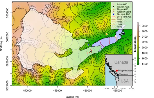
Bridge Glacier (50◦48′11′′N, 123◦38′40′′W), an outlet of the Lillooet Icefield, is lo-cated in the Pacific Ranges of the Coast Mountains of southwestern British Columbia, Canada, roughly 175 km north of Vancouver. The glacier had an area of 83 km2as of the end of the 2013 melt season, extending from an elevation of over 2900 m at Bridge
20
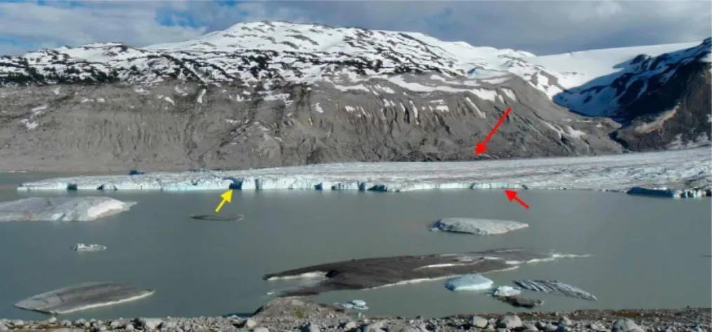
Peak, to 1390 m, where it terminates in a proglacial lake, locally known as Bridge Lake (see Fig. 1). The lake has grown from under 2 km2 in 1972 to over 6 km2 in 2013 as the glacier retreated across an overdeepened basin. The glacier has experienced large tabular calving events since the early 1990s, indicative of a floating terminus. The far (east) end of the lake traps numerous large (several hundred m2) icebergs which are
25
TCD
9, 2915–2953, 2015The relative contributions of calving and surface
ablation
M. Chernos et al.
Title Page
Abstract Introduction
Conclusions References
Tables Figures
◭ ◮
◭ ◮
Back Close
Full Screen / Esc
Printer-friendly Version Interactive Discussion
Discussion
P
a
per
|
Discussion
P
a
per
|
Discussion
P
a
per
|
Discussion
P
a
per
|
Bridge Glacier lies on the divide between the humid coastal Pacific Ranges and the drier interior Chilcotin Ranges. Synoptic air flow is predominantly from the west, generating heavy snowfall on the highest elevation, most westerly areas, while the eastern flank of the glacier is drier, with a mean May 1 SWE of 600 mm (BC Ministry of Environment, 2014).
5
The annual retreat of Bridge Glacier, derived from delineations of the terminus us-ing repeat Landsat imagery since 1972 (Fig. 2), is comprised of several stages. Re-treat was slow prior to 1991, characterized by small calving events along the shal-low proglacial lake margin. The average rate of retreat between 1972 and 1991 was 21 m a−1, but accelerated to 144 m a−1 after 1991, punctuated by high annual retreat
10
rates followed by years of relative terminus stability, and the appearance of large tabu-lar icebergs in the lake. The rate of retreat accelerated again after 2009 to∼400 m a−1 (Fig. 3e).
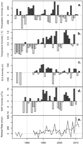
The substantial retreat that Bridge Glacier has undergone since 1991 cannot be fully explained by regional climate indicies (Fig. 3). For instance, from 1988 to 1998,
15
summer temperatures, equilibrium line altitudes, and discharge from Bridge Lake were all above the 30 year average (Fig. 3a–d), suggesting above average melting of the glacier surface. This period of elevated conditions for melt did not continue into the 21st century, however, retreat continued to accelerate. Since the mid-1990s, it appears that retreat was decoupled from climate. While it is clear the acceleration of retreat as
20
of 1991 is largely due to accelerated rates of calving, it remains unclear to what extent calving contributed to the total volume of ice loss from Bridge Glacier over the past 30 years.
3 Field methods
Three automatic weather stations (AWS) collected data from 20 June to 12 September
25
temper-TCD
9, 2915–2953, 2015The relative contributions of calving and surface
ablation
M. Chernos et al.
Title Page
Abstract Introduction
Conclusions References
Tables Figures
◭ ◮
◭ ◮
Back Close
Full Screen / Esc
Printer-friendly Version Interactive Discussion
Discussion
P
a
per
|
Discussion
P
a
per
|
Discussion
P
a
per
|
Discussion
P
a
per
|
ature, humidity, wind speed and direction, and reflected shortwave radiation at 10 min intervals. A second weather station (Ridge AWS), installed on a ridge∼250 m above the glacier toe and hence shielded from strong, persistent katabatic flow, collected am-bient temperature and solar radiation. A third weather station, located along the shore of Bridge Lake (Lake AWS) approximately 3 km from the terminus, on a partially
sub-5
merged end moraine, measured incoming longwave radiation, air temperature, humid-ity, wind speed, and rainfall. Rainfall was also measured at an exposed nunatak north of the main arm of the glacier (Nunatak TLC), to estimate the precipitation gradient over the glacier tongue.
In order to ground-truth surface melt derived from from melt modelling, 3 m-long
ab-10
lation stakes were installed at six locations in the ablation area. Due to logistical chal-lenges, and to obtain results that could also be used to ground-truth velocity estimates, the stakes were located within 2 km of the terminus (Fig. 1). The stakes were installed on 18 June, and resurveyed on 19 July and 13 September 2013.
The bathymetry of Bridge Lake was collected using a Lowrance HDS Gen2
depth-15
sounder, with a depth range of 500 m and horizontal GPS accuracy of ±5 m. Depth measurements were taken at 893 discrete points in an irregular grid. Access to the terminus and the middle part of the lake was hindered by the presence of icebergs. An additional 74 points were added by linear interpolation using known depths along east-west transects to improve coverage. The bathymetric data were processed using
20
the gstat package in R (R Core Team, 2013; Pebesma, 2004), and interpolated onto a 10 m grid using inverse distance weighting.
The change in terminus area during the study period was computed from Landsat images on 23 June and 11 September 2013. Shapefiles for both scenes were gener-ated by manually delineating the terminus in Google Earth. The change in area was
25
then calculated using the rgeos package in R.
TCD
9, 2915–2953, 2015The relative contributions of calving and surface
ablation
M. Chernos et al.
Title Page
Abstract Introduction
Conclusions References
Tables Figures
◭ ◮
◭ ◮
Back Close
Full Screen / Esc
Printer-friendly Version Interactive Discussion
Discussion
P
a
per
|
Discussion
P
a
per
|
Discussion
P
a
per
|
Discussion
P
a
per
|
video analysis and modelling tool (Brown, 2014). Raw pixel displacement was con-verted into distances using known camera angles and several ground control points. Eight points in close proximity on the glacier surface (<200 m) were tracked from each camera throughout the study period using daily noon-time images. Filtering routines discarded roughly 10 % of the tracked data points due to negative displacement, or loss
5
of target. Daily surface velocities were generated by averaging the daily displacements for each tracked point, and the average summer velocity was calculated by averaging the total displacement for each tracked point throughout the study period. Study-period time-lapse velocity measurements were complemented with an end-of-summer survey of ablation stakes; results were found to agree within the error of our Garmin eTrex
10
GPS (±5 m).
4 Modelling surface melt
Elevation data for the glacier surface were obtained using a 25 m resolution LIDAR dig-ital elevation model (from C-CLEAR by M. Demuth, C. Hopkinson, and B. Menounos, see Acknowledgements). The DEM was resampled to 50 m to reduce computation time
15
and digital artifacts in the data. To obtain historical estimates of surface melt, annual terminus retreat and equilibrium line altitudes (ELAs) were reconstructed from satellite imagery, using Landsat images from 1984 to 2012. All Landsat data were taken from images between 12 September and 24 October to represent end-of-season snowlines. The volume of ice lost by surface melt during the 2013 summer season was
com-20
puted with a distributed energy balance model using the data from the three AWS and the digital elevation model of the glacier surface. Surface melt of ice (M), in m (w.e.) d−1, was calculated as
M= QM
Lfρi
TCD
9, 2915–2953, 2015The relative contributions of calving and surface
ablation
M. Chernos et al.
Title Page
Abstract Introduction
Conclusions References
Tables Figures
◭ ◮
◭ ◮
Back Close
Full Screen / Esc
Printer-friendly Version Interactive Discussion
Discussion
P
a
per
|
Discussion
P
a
per
|
Discussion
P
a
per
|
Discussion
P
a
per
|
whereQMis the sum of available energy at the surface (W m
−2
),Lf is the latent heat of
fusion (3.34×10⁶J kg−1), andρi is the density of ice (917 kg m
−3
). Energy supplied to the glacier surface is positive, while energy flux away from the surface is negative. The available energy for melt was calculated as
QM=Q∗+QH+QE+QR (2)
5
whereQ∗is the net radiation,QHandQEare the sensible and latent heat flux, andQRis sensible heat of rain. All energy fluxes are in W m−2. We assume that all energy fluxes occur at the ice surface (Oerlemans, 2010; Munro, 2006); subsurface and subglacial melt is neglected.
4.1 Snowline retreat
10
As our purpose was to calculate the total ice loss during the melt season only, we only consider ice melt and not snowmelt, and hence the model was only applied to the glacier surface below the snowline at each time step. In order to calculate the volume of ice melt at each time step, snowline retreat over the course of the summer melt season was reconstructed from nine Landsat images obtained from the LandsatLook
15
Viewer (U. S. Geological Survey, 2014) between 1 June and 19 September 2013. Mul-tiple measurements of snowline altitude across the glacier surface were taken for each image, and averaged to produce a basin-wide snowline elevation. Temporal interpola-tion between snowline elevainterpola-tions was achieved using the loess smoothing funcinterpola-tion in R. The snowline was at the terminus until 15 June, and the ablation area had become
20
TCD
9, 2915–2953, 2015The relative contributions of calving and surface
ablation
M. Chernos et al.
Title Page
Abstract Introduction
Conclusions References
Tables Figures
◭ ◮
◭ ◮
Back Close
Full Screen / Esc
Printer-friendly Version Interactive Discussion
Discussion
P
a
per
|
Discussion
P
a
per
|
Discussion
P
a
per
|
Discussion
P
a
per
|
4.2 Net radiation
Net radiation (Q∗) is calculated as the sum of incoming (↓) and outgoing (↑) shortwave and longwave (L) radiation as follows:
Q∗=(S↓+D↓)(1−α)+(L↓ −L↑) (3)
where shortwave radiation (K) is separated into direct (S) and diffuse (D) components,
5
andα is the albedo of ice.
Reflected shortwave radiation was measured on-glacier and on bare ice in the ab-lation area, throughout the melt season. Incoming shortwave radiation was measured from the off-glacier Ridge AWS. Differences in shading between the two sites were found to be negligible. To minimize the effects of small discrepancies in shading,
un-10
even cloud patterns, and low solar angle errors (Oerlemans, 2010), the daily ice albedo (α) is assumed constant throughout the day, and is calculated as
α=
Z
K ↑dt/
Z
K ↓dt (4)
where the integrals are over the period of daylight each day.
Direct shortwave radiation (W m−2) for each gridpoint on the glacier surface is
calcu-15
lated as
S↓i,j=S↓
Kexi,j
Kex (5)
whereKexi,j is the potential direct solar radiation at grid point (i,j) andKexis the
poten-tial direct solar radiation at Glacier AWS. Measured global radiation was separated into direct and diffuse components based on the ratio of observed to potential shortwave
20
TCD
9, 2915–2953, 2015The relative contributions of calving and surface
ablation
M. Chernos et al.
Title Page
Abstract Introduction
Conclusions References
Tables Figures
◭ ◮
◭ ◮
Back Close
Full Screen / Esc
Printer-friendly Version Interactive Discussion
Discussion
P
a
per
|
Discussion
P
a
per
|
Discussion
P
a
per
|
Discussion
P
a
per
|
and Flowers, 2011) as
Di,j =Doφi,j+αterrainK ↓(1−φi,j) (6) whereDois the global diffuse radiation, corrected using the sky view factor (φ) for each
grid cell.
Due to the complications and heterogeneity involved in measuring the albedo for
5
the surrounding non-glaciated terrain (αterrain), a constant value of 0.17 was assumed,
which is within the range for dark, rocky surfaces (Oke, 1988). Sky view factor was calculated using SAGA GIS software and a 25 m lidar DEM. The algorithm integrates the maximum horizon angles (H) for each grid cell, for each azimuth angle (1◦interval). A maximum 10 km×10 km search window was implemented to reduce computation
10
time.
In order to spatially distribute incoming shortwave radiation, each grid point is mod-elled as either shaded or sunlit. A shading algorithm was implemented that calculates the maximum horizon angle for each grid point within a 10 km×10 km window, using 10◦ azimuth bins. At each time step, if the horizon angle is greater than the elevation
15
angle (Z), the grid point is shaded, and only receives diffuse radiation. For times when the horizon angle is smaller than elevation angle, the grid point receives both direct and diffuse radiation.
Incoming longwave radiation was measured directly at the Lake AWS. In order to distribute longwave radiation across the glacier, it is scaled by the sky view factor (φ)
20
as
L↓i,j =L↓aws
φi,j
φaws
+Lterrain(1−φi,j) (7)
where additional longwave input is supplied by the surrounding terrain (Lterrain). Terrain
TCD
9, 2915–2953, 2015The relative contributions of calving and surface
ablation
M. Chernos et al.
Title Page
Abstract Introduction
Conclusions References
Tables Figures
◭ ◮
◭ ◮
Back Close
Full Screen / Esc
Printer-friendly Version Interactive Discussion
Discussion
P
a
per
|
Discussion
P
a
per
|
Discussion
P
a
per
|
Discussion
P
a
per
|
4.3 Turbulent heat fluxes
Sensible and latent heat fluxes are calculated using the bulk transfer approach:
QH=ρaircaCu(Tg−Ts) (8)
QE=ρairLvCu
0.622(eg−es)
P
!
(9)
where cair is the specific heat capacity of air (1006 J kg
−1
K−1), u is the windspeed
5
(m s−1),Tgis the on-glacier air temperature,Tsis the glacier surface temperature (held
constant at 273.15 K),Lv is the latent heat of vaporization (2.50 ×10 6
J kg−1),eg and
esare the vapour pressures (hPa) of air and glacier surface (held constant at 6.11 hPa,
assuming the glacier surface is at the melting point), andP is the atmospheric pres-sure (hPa) at Glacier AWS. The turbulent transfer coefficientC(unitless) is calculated
10
using bulk Richardson Numbers, using a roughness length for momentum of 2.5 mm for ice (Munro, 1989), and calculating the roughness length for temperature and vapour following Hock (1998).
Air temperature was distributed over the glacier surface using the approach devel-oped by Shea and Moore (2010), which accounts for the effects of katabatic flow. In
15
this approach, the magnitude of katabatic forcing was modelled as a function of the temperature difference (∆T) between the on-glacier Glacier AWS (Tg) and off-glacier
Ridge AWS (Ta, outside the katabatic boundary layer). Temperature differences were
separated into upslope (northeasterly) and downslope katabatic (southwesterly) flows, based on the wind directions of Glacier AWS. Linear regression against off-glacier
tem-20
perature (Ta, Fig. 4) shows a positive linear increase in∆T, indicating the magnitude of
katabatic forcing increases with increasing off-glacier air temperatures. Conversely,∆T
TCD
9, 2915–2953, 2015The relative contributions of calving and surface
ablation
M. Chernos et al.
Title Page
Abstract Introduction
Conclusions References
Tables Figures
◭ ◮
◭ ◮
Back Close
Full Screen / Esc
Printer-friendly Version Interactive Discussion
Discussion
P
a
per
|
Discussion
P
a
per
|
Discussion
P
a
per
|
Discussion
P
a
per
|
both weather stations are within 100 m, and small corrections to potential temperature using a−6◦C km−1lapse rate did not produce a meaningful difference in the linear fit.
On-glacier air temperature for each grid point is modelled as a function of the kata-batic temperature depression where
Tg=Ta−(k1Ta+ ∆T∗) (10)
5
and∆T∗ is the threshold temperature differential at which katabatic flow is observed. The magnitude of katabatic forcing for each point on the glacier,k1, is calculated using
statistical coefficients and glacier flow path lengths (Shea, 2010; Chernos, 2014). Flow path lengths for the glacier were calculated using the Terrain Analysis – Hydrology module of SAGA GIS (Quinn et al., 1991; SAGA Development Team, 2008). During
10
periods when wind direction is upslope, temperatures are distributed using the on-glacier temperature,Tg, and a standard temperature lapse rate of−6
◦
C km−1.
Wind speed across the glacier was distributed as a function of katabatic forcing and ambient temperatures, following Shea (2010). For situations when the measured on-glacier wind direction was downslope, wind speed increases linearly with increasing
15
off-glacier air temperature, while upslope wind speeds show no significant change. When the measured on-glacier wind direction is upslope, wind speed is held constant, using measured wind speeds from Glacier AWS.
Vapour pressure is calculated from measured relative humidity and saturation vapour pressure (esat). Relative humidity, measured at Glacier AWS, is held spatially constant 20
across the glacier for each timestep, and saturation vapour pressure is calculated from distributed on-glacier air temperatures.
4.4 Melt contribution from rain
Energy supplied to the surface due to rain was calculated as
QR=ρwcwRTR (11)
TCD
9, 2915–2953, 2015The relative contributions of calving and surface
ablation
M. Chernos et al.
Title Page
Abstract Introduction
Conclusions References
Tables Figures
◭ ◮
◭ ◮
Back Close
Full Screen / Esc
Printer-friendly Version Interactive Discussion
Discussion
P
a
per
|
Discussion
P
a
per
|
Discussion
P
a
per
|
Discussion
P
a
per
|
whereR is the rainfall rate (m s−1), measured at the Lake AWS (and missing values are filled with measured data from Nunatak TLC), and ρw and cw are the density
(1000 kg m−3) and specific heat of water (4180 J kg−1K−1). The temperature of rain,
TR, is assumed equal to the ambient off-glacier air temperature, and is corrected for
elevation using a standard lapse rate.
5
5 Modelling calving flux
Calving losses are calculated from measured retreat rates and flow speeds, as well as estimates of ice thickness derived from bathymetry. The volume of ice discharged through calving from the glacier terminus,Qcalving(m
3
a−1), i.e., the calving flux, can be quantified as
10
Qcalving=
dA T
dt +UW
HI (12)
where dAT
d t is the change in glacier surface area at the terminus (m
2
a−1), U is the terminus flow velocity (m a−1), HI and W are the ice thickness (m) and glacier width
(m) at the terminus. Subaqueous melt at the ice front is assumed to be negligible with respect to the magnitude of the calving flux.
15
The thickness of ice at the terminus was approximated by assuming that the terminus is floating. Using the height above buoyancy criterion (Van der Veen, 1996; Benn et al., 2007b), the ice thickness (HI) can be calculated as
HI=Hb+
ρw
ρi
DW (13)
whereHb is the height of ice above the waterline (m),DWis the water depth, while ρw 20
andρiare the densities of water and ice. The validity of this assumption is supported by
TCD
9, 2915–2953, 2015The relative contributions of calving and surface
ablation
M. Chernos et al.
Title Page
Abstract Introduction
Conclusions References
Tables Figures
◭ ◮
◭ ◮
Back Close
Full Screen / Esc
Printer-friendly Version Interactive Discussion
Discussion
P
a
per
|
Discussion
P
a
per
|
Discussion
P
a
per
|
Discussion
P
a
per
|
limited mobility immediately after calving, suggesting that the glacier is close to the boundary criterion for flotation. There is a notable inflection point (Fig. 5), where it is assumed that the terminus transitions from grounded to floating.
The calving flux between 1984 and 2012 was computed from historical terminus po-sitions, lake bathymetry (Fig. 6), estimated ice thickness, and measured velocity from
5
the 2013 field season. Historical terminus velocities were assumed to be approximately equal to the 2013 summer flow speed (140 m a−1), and annual calving rates are calcu-lated with 70 m a−1(50 %) potential variability around the 2013 mean.
From the repeat Landsat imagery, it is clear that the terminus became ungrounded and achieved flotation around 1991. Given that terminus velocities are presumed to be
10
a function of basal drag (Benn et al., 2007a), once the terminus achieved flotation it is likely that terminus flow speeds have not changed dramatically since then. However, we recognize that terminus velocities were likely slower when the calving front was grounded, and hence we are likely overestimating calving rates prior to 1991.
A 60 m uncertainty in measuring the terminus cross-section (W) (equal to 2 Landsat
15
pixels) is applied. The uncertainty ofddAt is estimated as 7200 m2a−1(2 m×60 m×60 m). The ice thickness uncertainty is estimated as 5.6 % plus an additional 10 m to account for changes in sedimentation and ice thickness relative to water depth. Before 1991, the terminus was not floating; therefore, an ice thickness uncertainty of 60 m is esti-mated to account for a range of grounded terminus geometries. Between 1991 and
20
2004, bathymetry has poor data coverage, and a ice thickness uncertainty of 33 m is estimated.
6 Historical surface melt
In order to understand the long-term mass loss at Bridge Glacier, estimates of histori-cal surface melt are derived using ELA observations and a fitted linear mass balance
25
gradient (Shea et al., 2013). Below the snowline, the net balance (wherebn=bw+bs)
TCD
9, 2915–2953, 2015The relative contributions of calving and surface
ablation
M. Chernos et al.
Title Page
Abstract Introduction
Conclusions References
Tables Figures
◭ ◮
◭ ◮
Back Close
Full Screen / Esc
Printer-friendly Version Interactive Discussion
Discussion
P
a
per
|
Discussion
P
a
per
|
Discussion
P
a
per
|
Discussion
P
a
per
|
where
bn(z)=b1(ELA−z) (14)
and is calculated for the elevation of every point,z (m a.s.l.), below the ELA. The coefficient value (b1=6.62 m (w.e.) m
−1
) taken from Shea et al. (2013) under-estimates the volume of ice loss during the 2013 melt season calculated from the
5
distributed energy balance model. Coefficient b1 is derived from the mass balance
gradient from the DEBM (9.07 m (w.e.) m−1, Fig. 7), and is used for all years.
The glacier area is determined from the end-of-season calving margin. Calved area is given an elevation of 1400 m (a.s.l.) and are considered in Eq. (14). Historical ELAs are measured from end-of-summer (mid-September to mid-October) Landsat images
10
from 1984 to 2013.
Errors in ELA-derived mass balance calculations are estimated by assuming a 75 m uncertainty in measuring the ELA, due to timing of available Landsat images, or 22 % according to Shea et al. (2013), whichever is greater. The ELA uncertainty estimate is to account for errors that cannot be adequately quantified without additional historical
15
data, such as the linearity of the mass balance gradient.
7 Results
7.1 The 2013 surface melt
From 20 June to 12 September 2013, our model predicted 1.0 m (w.e.) of surface ice loss of near the ELA to 5.9 m (w.e.) near the terminus, yielding a total mass loss of
20
0.124 km3(Fig. 8). Melt rates are greatest along the main tongue of the glacier, due to high sensible heat flux driven by persistent katabatic flow. The southernmost tributary glacier shows relatively low melt rates relative to its elevation, most likely due to the fact that it remained sheltered from high winds and its north-facing aspect allowed for substantial shading throughout the melt season.
TCD
9, 2915–2953, 2015The relative contributions of calving and surface
ablation
M. Chernos et al.
Title Page
Abstract Introduction
Conclusions References
Tables Figures
◭ ◮
◭ ◮
Back Close
Full Screen / Esc
Printer-friendly Version Interactive Discussion
Discussion
P
a
per
|
Discussion
P
a
per
|
Discussion
P
a
per
|
Discussion
P
a
per
|
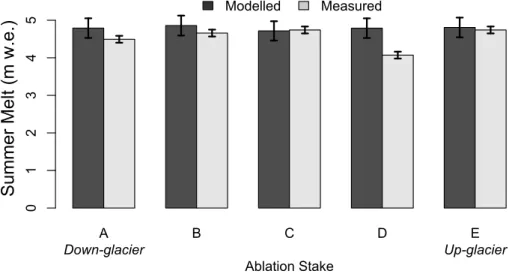
Modelled melt agreed within±0.2 m w.e. for four of the five ablation stakes (Fig. 9), representing an error of less than 5 % of the measured value. Measured melt at ablation stake D, located roughly 400 m up-glacier (∼100 m increase in elevation) from Glacier AWS and stake A, is up to 0.8 m less than other nearby stakes (including stake E, which is 200 m higher in elevation, and further up-glacier), suggesting that there may
5
have been errors in measurement, or localized effects shielding the stake from higher melt rates observed elsewhere in the ablation area.
7.2 The 2013 calving flux
The terminus retreated 65 m over 85 days in 2013, with a change in terminus area of
−0.297 km2. The average velocity at the terminus was 139 m a−1, across a width of
10
1055 m, yielding an additional loss of 0.0342 km2due to calving.
Water depth was estimated from a cross-section parallel to, and roughly 500 m from, the June 2013 terminus position. The median depth was 109 m, corresponding to a height above buoyancy of 9.9 m, and an estimated ice thickness of 109 m. Com-bining these measurements in Eq. (12) yields an estimated calving flux of 0.0362 km3
15
for the 85 day study period.
Comparing the volume of mass lost through calving with the volume of surface ice melt during the same period yields a total mass loss of 0.160 km3of ice. For the 2013 melt season, calving accounts for 23 % of the mass loss, equivalent to an additional 1.3 m of surface melt over the entire ablation area.
20
7.3 Historical ice loss
The volume of ice lost from surface melt over the past 30 years was predominantly a function of the position of the ELA, and showed only a minor decrease over time. Between 1984 and 2013, the ELA varied from 1926 to 2202 m; however, in most years the ELA was between 2050 and 2150 m, resulting in a standard deviation in volumetric
25
TCD
9, 2915–2953, 2015The relative contributions of calving and surface
ablation
M. Chernos et al.
Title Page
Abstract Introduction
Conclusions References
Tables Figures
◭ ◮
◭ ◮
Back Close
Full Screen / Esc
Printer-friendly Version Interactive Discussion
Discussion
P
a
per
|
Discussion
P
a
per
|
Discussion
P
a
per
|
Discussion
P
a
per
|
but within one standard deviation of the mean (x=0.107 km3). Surface melt showed a minor decrease over time, which can be attributed to the loss of surface area in the lowest reaches of the glacier due to calving and retreat.
Historical calving losses are characterized by several years of high flux, and peri-ods of relative stability. The magnitude of the calving losses increased once the glacier
5
achieved flotation in 1991. Calving losses are minimal before 1991, most likely due to the relative stability of a grounded terminus. From 1992 to 1994, the calving flux in-creased to 0.020–0.029 km3(19–27 % of the total annual ice loss), before a two year period of low flux (<0.015 km3). From 1997 to 2000, calving losses increased again (0.023–0.052 km3), before settling into another period of relative stability in 2001–2002.
10
The highest calving fluxes occurred between 2003 to 2006 (0.030–0.084 km3) and again from 2008 to 2011 (0.036–0.100 km3) with a period of stability in 2006–2007. As the calving flux increased in the period from 2003–2011, surface ablation rates de-creased, resulting in the calving flux becoming a larger component of total ice loss in the 21st century. The volume of ice loss due to calving was roughly equal to the
vol-15
ume lost due to surface melt in 2005, 2008 and 2010 (44–49 % of total volumetric ice losses).
8 Discussion
8.1 Controls on calving
During the 2013 melt season, calving was a moderate contributor of mass loss relative
20
to surface melt at Bridge Glacier. Calving losses in this system are controlled by glacio-logical and topographical controls that ultimately limit the magnitude of the calving flux. The glacier width at the calving margin was just over 1 km, which restricts the volume of ice that can reach the floating terminus, in turn limiting the size of calving events. In contrast, the ablation area in 2013 was over 27.6 km2, allowing for surface melt
TCD
9, 2915–2953, 2015The relative contributions of calving and surface
ablation
M. Chernos et al.
Title Page
Abstract Introduction
Conclusions References
Tables Figures
◭ ◮
◭ ◮
Back Close
Full Screen / Esc
Printer-friendly Version Interactive Discussion
Discussion
P
a
per
|
Discussion
P
a
per
|
Discussion
P
a
per
|
Discussion
P
a
per
|
cesses to act over a much larger area and contribute a substantially larger volume of ice loss than possible from the calving front.
Relatively modest glacier flow speeds at the terminus also limit the volume of ice delivered to the terminus and calving. Flow velocity at Bridge Glacier is moderate due to gentle gradients in the lower reaches of the glacier, as well as relatively narrow
side-5
walls. A gentle surface slope reduces the gravitational stresses, while narrow valley sidewalls provide substantial lateral drag (Benn et al., 2007a; Koppes et al., 2011), both of which limit flow speeds. Near-terminus flow speeds at Bridge Glacier are one to two orders of magnitude smaller than those observed at larger tidewater calving glaciers in Patagonia and Alaska (Rivera et al., 2012; Koppes et al., 2011; Meier and
10
Post, 1987), and reflect a more stable character and configuration, similar to lake-terminating glaciers Mendenhall and Tasman (Boyce et al., 2007; Dykes et al., 2011).
Although water depths increased substantially during the highest rates of calving in the late 2000s, we do not expect major changes in terminus velocity since the terminus achieved floatation in 1991. The 2013 mean terminus water depth was within 15 m of
15
depths during the late 2000s, and was larger than the average water depth between 2004 and 2012. Given the relative consistency in water depths, and that the terminus is assumed to have remained floating throughout this most recent stage of retreat, we do not expect large changes in resisting stresses. Furthermore, a first order examination of thinning rates using Landsat images from the last two decades does not reveal major
20
year to year changes, suggesting that basal shear stresses, and hence velocities, have not varied significantly during this time. However, maximum water depths peaked in the mid-2000s, meaning that is is possible that velocities could have been higher during this period (Van der Veen, 1996), making our calving fluxes underestimates. Conversely, it is likely that pre-1991 velocities were substantially smaller than what was measured in
25
2013. As such, it is unlikely that calving losses could equal the upper bounds of our estimate during this pre-floatation period.
TCD
9, 2915–2953, 2015The relative contributions of calving and surface
ablation
M. Chernos et al.
Title Page
Abstract Introduction
Conclusions References
Tables Figures
◭ ◮
◭ ◮
Back Close
Full Screen / Esc
Printer-friendly Version Interactive Discussion
Discussion
P
a
per
|
Discussion
P
a
per
|
Discussion
P
a
per
|
Discussion
P
a
per
|
thickness at the terminus and the water depth. Any significant thickening of the glacier, without any concurrent increase in lake level, would theoretically increase the poten-tial volume of ice lost to calving, but would also serve to reduce the buoyancy of the terminus and allow the terminus to become grounded. Grounding would stabilize the terminus, and significantly reduce potential calving losses. In other words, any increase
5
in terminus thickness is more likely to reduce, rather than enhance, the calving flux.
8.2 The relative importance of calving
From 1984 to 2013, the calving flux increased from an almost negligible annual yield to a flux responsible for between 20–45 % of the annual ice loss. The trend in calving flux closely follows water depth at the terminus, where the largest calving fluxes coincide
10
with the terminus retreating into the deepest parts of Bridge Lake in 2003–2011. This relationship suggests that buoyancy is a primary driver of calving at Bridge Glacier. It also implies that the high rate of calving currently observed is unsustainable over the coming decades, and is instead part of a transient phase as the glacier continues to retreat up-valley and into shallower waters.
15
Although calving contributed less than one quarter of the total ice loss from Bridge Glacier during the 2013 melt season, during three of the last ten years the volume of ice loss due to calving is on par with the volume lost due to surface melt. However, large annual calving fluxes do not persist over several consecutive seasons, and are instead followed by several years of only minor calving losses, even though the terminus
re-20
mained in the deepest part of the lake. The pattern of a high magnitude calving year followed by several low-flux years is consistent with the notion that glacier dynamics respond to large calving events by alleviating terminus instability and inhibiting future calving (Venteris, 1999; Benn et al., 2007b). Following a large calving event, the glacier geometry changes, and buoyant forces can be redistributed or relieved, promoting
ter-25
minus stability.
TCD
9, 2915–2953, 2015The relative contributions of calving and surface
ablation
M. Chernos et al.
Title Page
Abstract Introduction
Conclusions References
Tables Figures
◭ ◮
◭ ◮
Back Close
Full Screen / Esc
Printer-friendly Version Interactive Discussion
Discussion
P
a
per
|
Discussion
P
a
per
|
Discussion
P
a
per
|
Discussion
P
a
per
|
has produced substantial ice losses during the last 10 years, calving fluxes in most calving systems are driven by deep water and/or high flow speeds (Warren and Aniya, 1999; Van der Veen, 2002; Benn et al., 2007b). Given the lake bathymetry, and ob-served flow speeds at Bridge Glacier, it is unlikely that the terminus will remain in deep water for many more years, suggesting that current calving losses are transient, and
5
unsustainable. The primary contribution of surface melt to Bridge Glacier’s mass loss suggests that the glacier’s future health is more dependent on climatic conditions rather than calving losses, and surface melt is expected to become even more important as the glacier nears the end of this transient calving phase.
8.3 Bridge Glacier and other lake-calving systems
10
Bridge Glacier falls in the middle of a continuum of magnitude and frequency of calving in other lake-terminating glaciers worldwide (see Table 1). The calving rate for Bridge Glacier (281 m a−1 in 2013) is larger than that for smaller glaciers in New Zealand, such as Maug, Grey and Hooker (Warren and Kirkbride, 2003), and for Mendenhall Glacier in Alaska (Motyka et al., 2003; Boyce et al., 2007). Conversely, calving rates
15
at the larger Patagonian glaciers Leon, Ameghino, and Upsala are up to an order of magnitude greater than what we found at Bridge (Warren and Aniya, 1999).
Bridge Glacier’s calving rate is controlled by moderate water depths and flow speeds. Higher calving rates are associated with greater water depths and significantly larger terminus velocities. Large Patagonian and Icelandic glaciers have terminus
veloci-20
ties of up to 1810 m a−1 (Haresign, 2004), an order of magnitude greater than what we measured at Bridge Glacier (140 m a−1). Conversely, smaller calving glaciers in New Zealand terminate in shallow lakes (<50 m) and many have low flow speeds (<70 m a−1). Bridge Glacier’s calving rate in 2013 (281 m a−1) also agrees quite well with first-order linear models relating calving to water depth (Funk and Röthlisberger,
25
TCD
9, 2915–2953, 2015The relative contributions of calving and surface
ablation
M. Chernos et al.
Title Page
Abstract Introduction
Conclusions References
Tables Figures
◭ ◮
◭ ◮
Back Close
Full Screen / Esc
Printer-friendly Version Interactive Discussion
Discussion
P
a
per
|
Discussion
P
a
per
|
Discussion
P
a
per
|
Discussion
P
a
per
|
spectrum of calving and water depth for lake-calving glaciers worldwide, which is an order of magnitude lower than calving rates from tidewater systems (Fig. 12).
Lake temperatures also appear to play a role in controlling the calving rate. Many Patagonian icefields terminate in large lakes where water temperatures are up to 7.6◦C (Warren and Aniya, 1999), significantly warmer than the well-mixed 1◦C water
ob-5
served at Bridge Lake (Bird, 2014). This difference is most likely related to the sur-face area of the proglacial lakes. Bridge Lake is relatively large (6.3 km2), but is small relative to the much larger lakes of Southern Patagonia, that are greater than 300 m deep. This depth, combined with large areas that are free of the strong cooling influ-ence of glacier runoffand trapped icebergs, allows for these proglacial lakes to warm
10
significantly, and promote further calving.
Bridge Glacier shares similar calving characteristics with both Tasman and Menden-hall Glaciers, both of which have undergone significant retreat as they transitioned from grounded to floating termini (Boyce et al., 2007; Dykes et al., 2011). During this transition, terminus velocities increased at Tasman from 69 to 218 m a−1 (Dykes and
15
Brook, 2010; Dykes et al., 2011), while the calving rates for both glaciers increased from 50 m a−1to between 227 and 431 m a−1(Boyce et al., 2007; Dykes et al., 2011); these rates are consistent with what we found at Bridge Glacier. For both Tasman and Mendenhall Glaciers, water depth and buoyancy also control the magnitude of calving (Boyce et al., 2007; Dykes et al., 2011; Dykes, 2013), suggesting that the majority of
20
the ice discharged from the terminus is triggered by buoyant forces. As the multi-annual calving rate is driven primarily by water depth, unless glacier flow speeds remain high enough to continually transport ice to deeper lake waters, and maintain terminus flota-tion, the glacier will retreat into shallow water and regain stability.
9 Conclusions
25
TCD
9, 2915–2953, 2015The relative contributions of calving and surface
ablation
M. Chernos et al.
Title Page
Abstract Introduction
Conclusions References
Tables Figures
◭ ◮
◭ ◮
Back Close
Full Screen / Esc
Printer-friendly Version Interactive Discussion
Discussion
P
a
per
|
Discussion
P
a
per
|
Discussion
P
a
per
|
Discussion
P
a
per
|
1991. This retreat was independent of regional warming trends, and was enhanced by significant calving losses as the glacier terminus retreated into deeper waters. While calving has accelerated Bridge Glacier’s retreat, estimates of surface melt and the calving flux for the 2013 melt season indicate that calving was only responsible for 23 % of the total ice loss. The contribution of calving to mass loss was limited by modest
5
terminus flow speeds, relatively narrow side-walls in the lower glacial tongue, and lake depth at the terminus.
Estimates of calving and surface melt rates from 1984 to present suggest that calving did not contribute to significant mass loss before 1991. From 1991 to 2003 calving rates increased significantly, and the calving flux was on par with the volumetric ice loss
10
from surface melt in 2005, 2008 and 2010. Although individual years can have large calving fluxes, multi-year averages show that calving only contributed between 10 and 25 % of the total ice loss at Bridge Glacier. Therefore, the dominant control on the mass balance of Bridge Glacier is surface melt, and future projections of glacier retreat should be closely tied to climate. The rapid calving rates observed since 2009 at Bridge
15
Glacier are part of a transient stage in retreat as the glacier terminus passes through an overdeepened, lake-filled basin, and are not expected to remain a consistently large source of ice loss in the coming decades.
Acknowledgements. This work was supported financially by operating grants to M. Koppes
and R. D. Moore from the Natural Sciences and Engineering Research Council (NSERC) and
20
a Canada Foundation of Innovation Leaders Fund grant to M. Koppes. Assistance with field data collection was provided by Lawrence Bird, Alistair Davis, and Mélanie Ebsworth. The authors gratefully acknowledge M. Demuth, C. Hopkinson, and B. Menounos for the LiDAR data used in this study, which was collected as part of a C-CLEAR effort to develop LiDAR environmental applications, and funded in part by the Western Canadian Cryospheric Network (WCCN).
25
References
TCD
9, 2915–2953, 2015The relative contributions of calving and surface
ablation
M. Chernos et al.
Title Page
Abstract Introduction
Conclusions References
Tables Figures
◭ ◮
◭ ◮
Back Close
Full Screen / Esc
Printer-friendly Version Interactive Discussion
Discussion
P
a
per
|
Discussion
P
a
per
|
Discussion
P
a
per
|
Discussion
P
a
per
|
BC Ministry of Environment: Historic Snow Survey Data, available at: h9p://bcrfc.env.gov.bc.ca/ data/asp/archive.htm (last access: 30 September 2014), 2014. 2919
Benn, D., Hulton, N., and Mottram, R.: “Calving laws”, “sliding laws” and the stability of tidewater glaciers, Ann. Glaciol., 46, 123–130, 2007a. 2917, 2928, 2932
Benn, D., Warren, C., and Mottram, R.: Calving processes and the dynamics of calving glaciers,
5
Earth-Sci. Rev., 82, 143–179, 2007b. 2927, 2933, 2934
Bird, L.: Hydrology and Thermal Regime of a Proglacial Lake Fed by a Calving Glacier, M.S. thesis, University of British Columbia, Vancouver, Canada, 2014. 2935
Boyce, E. S., Motyka, R. J., and Truffer, M.: Flotation and retreat of a lake-calving terminus, Mendenhall Glacier, southeast Alaska, USA, J. Glaciol., 53, 211–224,
10
doi:10.3189/172756507782202928, 2007. 2917, 2932, 2934, 2935, 2941
Brown, D.: Tracker Video Analysis and Modeling Tool, available at: https://www.cabrillo.edu/ ~dbrown/tracker/ (last access: 1 February 2014), 2014. 2921
Chernos, M.: The Relative Importance of Calving and Surface Ablation at a Lacustrine Termi-nating Glacier, M.S. thesis, University of British Columbia, Vancouver, Canada, 2014. 2926,
15
2941
Collares-Pereira, M. and Rabl, A.: The average distribution of solar radiation-correlations be-tween diffuse and hemispherical and between daily and hourly insolation values, Sol. Energy, 22, 155–164, 1979. 2923
Cowie, N. M., Moore, R. D., and Hassan, M. A.: Effects of glacial retreat on proglacial streams
20
and riparian zones in the Coast and North Cascade Mountains, Earth Surf. Proc. Land., 39, 351–365, 2014. 2917
Dykes, R. C.: A Multi-Parameter Study of Iceberg Calving and the Retreat of Haupapa Tasman Glacier, South Island, New Zealand, Ph.D. thesis, Massey University, Palmerston North, New Zealand, 2013. 2935
25
Dykes, R. C. and Brook, M. S.: Terminus recession, proglacial lake expansion and 21st cen-tury calving retreat of Tasman Glacier, New Zealand, New Zeal. Geogr., 66, 203–217, doi:10.1111/j.1745-7939.2010.01177.x, 2010. 2917, 2935
Dykes, R., Brook, M., Robertson, C., and Fuller, I.: Twenty-first century calving retreat of Tasman Glacier, Southern Alps, New Zealand, Arct. Antarct. Alp. Res., 43, 1–10,
30
TCD
9, 2915–2953, 2015The relative contributions of calving and surface
ablation
M. Chernos et al.
Title Page
Abstract Introduction
Conclusions References
Tables Figures
◭ ◮
◭ ◮
Back Close
Full Screen / Esc
Printer-friendly Version Interactive Discussion
Discussion
P
a
per
|
Discussion
P
a
per
|
Discussion
P
a
per
|
Discussion
P
a
per
|
Dyurgerov, M. and Meier, M.: Glaciers and the Changing Earth System: a 2004 Snapshot, Institute of Arctic and Alpine Research, University of Colorado, Boulder, CO, 2005. 2916, 2917
Dyurgerov, M., Meier, M., and Armstrong, R. L.: Glacier Mass Balance and Regime: Data of Measurements and Analysis, Institute of Arctic and Alpine Research, University of Colorado,
5
Boulder, USA, 2002. 2916
Funk, M. and Röthlisberger, H.: Forecasting the effects of a planned reservoir which will partially flood the tongue of Unteraargletscher in Switzerland, Ann. Glaciol., 13, 76–81, 1989. 2934 Haresign, E.: Glacio-Limnological Interactions at Lake-Calving Glaciers, Ph.D. thesis, University
of St. Andrews, St. Andrews, Scotland, 2004. 2934, 2941, 2953
10
Hock, R.: Modelling of Glacier Melt and Discharge, Ph.D. thesis, ETH Zurich, Zurich, Switzer-land, 1998. 2925
Hock, R. and Holmgren, B.: A distributed surface energy-balance model for complex topography and its application to Storglaciären, Sweden, J. Glaciol., 51, 25–36, 2005. 2923
Kaser, G., Cogley, J., Dyurgerov, M., Meier, M., and Ohmura, A.: Mass balance of glaciers
15
and ice caps: Consensus estimates for 1961–2004, Geophys. Res. Lett., 33, L19501, doi:10.1029/2006GL027511, 2006. 2917
Koppes, M., Conway, H., Rasmussen, L. A., and Chernos, M.: Deriving mass balance and calving variations from reanalysis data and sparse observations, Glaciar San Rafael, north-ern Patagonia, 1950–2005, The Cryosphere, 5, 791–808, doi:10.5194/tc-5-791-2011, 2011.
20
2932
MacDougall, A. H. and Flowers, G. E.: Spatial and temporal transferability of a distributed energy-balance glacier melt model, J. Climate, 24, 1480–1498, 2011. 2923
Marshall, S., White, E., Demuth, M., Bolch, T., Wheate, R., Menounos, B., Beedle, M., and Shea, J.: Glacier water resources on the eastern slopes of the Canadian Rocky Mountains,
25
Can. Water Resour. J., 36, 109–134, 2011. 2917
Meier, M. and Post, A.: Fast tidewater glaciers, J. Geophys. Res., 92, 9051–9058, 1987. 2917, 2932
Milner, A. M. and Bailey, R.: Salmonid colonization of new streams in Glacier Bay National park, Alaska, Aquac. Res., 20, 179–192, 1989. 2917
30
run-TCD
9, 2915–2953, 2015The relative contributions of calving and surface
ablation
M. Chernos et al.
Title Page
Abstract Introduction
Conclusions References
Tables Figures
◭ ◮
◭ ◮
Back Close
Full Screen / Esc
Printer-friendly Version Interactive Discussion
Discussion
P
a
per
|
Discussion
P
a
per
|
Discussion
P
a
per
|
Discussion
P
a
per
|
off, Global Planet. Change, 35, 93–112, doi:10.1016/S0921-8181(02)00138-8, 2003. 2917, 2934, 2941
Munro, D. S.: Surface roughness and bulk heat transfer on a glacier: comparison with eddy correlation, J. Glaciol., 35, 343–348, 1989. 2925
Munro, D. S.: Linking the weather to glacier hydrology and mass balance at Peyto Glacier,
5
in: Peyto Glacier: One Century of Science, National Hydrology Research Institute Science Report, Otawa, Canada, 278, 135–178, 2006. 2922
Oerlemans, J.: Extracting a climate signal from 169 glacier records, Science, 308, 675–677, doi:10.1126/science.1107046, 2005. 2916, 2917
Oerlemans, J.: The Microclimate of Valley Glaciers, Igitur, Utrecht Publishing & Archiving
Ser-10
vices, Utrecht, the Netherlands, 2010. 2922, 2923
Oke, T.: Boundary Layer Climates, Routledge, London, England, 1988. 2924
Pebesma, E. J.: Multivariable geostatistics in S: the gstat package, Comput. Geosci., 30, 683– 691, 2004. 2920
Post, A., O’Neel, S., Motyka, R., and Streveler, G.: A complex relationship between calving
15
glaciers and climate, Eos, Trans. Am. Geophys. Union, 92, 305–312, 2011. 2917
Quinn, P., Beven, K., Chevallier, P., and Planchon, O.: The prediction of hillslope flow paths for distributed hydrological modelling using digital terrain models, Hydrol. Process., 5, 59–79, 1991. 2926
R Core Team: R: a Language and Environment for Statistical Computing, R Foundation for
20
Statistical Computing, Vienna, Austria, available at: http://www.R-project.org/ (last access: 15 April 2014), 2013. 2920
Rivera, A., Corripio, J., Bravo, C., and Cisternas, S.: Glaciar Jorge Montt (Chilean Patagonia) dynamics derived from photos obtained by fixed cameras and satellite image feature tracking, Ann. Glaciol., 53, 147–155, 2012. 2932
25
SAGA Development Team: System for Automated Geoscientific Analyses (SAGA GIS), Ger-many, available at: http://www.saga-gis.org/ (last access: 15 April 2014), 2008. 2926 Shea, J. M.: Regional-Scale Distributed Modelling of Glacier Meteorology and Melt, Southern
Coast Mountains, Canada, Ph.D. thesis, University of British Columbia, Vancouver, Canada, 2010. 2926
30
TCD
9, 2915–2953, 2015The relative contributions of calving and surface
ablation
M. Chernos et al.
Title Page
Abstract Introduction
Conclusions References
Tables Figures
◭ ◮
◭ ◮
Back Close
Full Screen / Esc
Printer-friendly Version Interactive Discussion
Discussion
P
a
per
|
Discussion
P
a
per
|
Discussion
P
a
per
|
Discussion
P
a
per
|
Shea, J. M., Menounos, B., Moore, R. D., and Tennant, C.: An approach to derive regional snow lines and glacier mass change from MODIS imagery, western North America, The Cryosphere, 7, 667–680, doi:10.5194/tc-7-667-2013, 2013. 2928, 2929, 2948
Stahl, K., Moore, R., Shea, J., Hutchinson, D., and Cannon, A.: Coupled modelling of glacier and streamflow response to future climate scenarios, Water Resour. Res., 44, W02422,
5
doi:10.1029/2007WR005956, 2008. 2917
Stuefer, M., Rott, H., and Skvarca, P.: Glaciar Perito Moreno, Patagonia: climate sensitivities and glacier characteristics preceding the 2003/04 and 2005/06 damming events, J. Glaciol., 53, 3–16, 2007. 2917, 2941
U.S. Geological Survey: LandsatLook Viewer, available at: http://landsatlook.usgs.gov/ (last
ac-10
cess: 1 September 2014), 2014. 2922
Van der Veen, C.: Tidewater calving, J. Glaciol., 42, 375–385, 1996. 2927, 2932 Van der Veen, C.: Calving glaciers, Prog. Phys. Geog., 26, 96–122, 2002. 2917, 2934
Venteris, E. R.: Rapid tidewater glacier retreat: a comparison between Columbia Glacier, Alaska and Patagonian calving glaciers, Global Planet. Change, 22, 131–138, 1999. 2933
15
Warren, C. and Aniya, M.: The calving glaciers of southern South America, Global Planet. Change, 22, 59–77, 1999. 2917, 2934, 2935, 2941
Warren, C. and Sugden, D.: The Patagonian Icefields: a glaciological review, Arctic Alpine Res., 75, 316–331, 1993. 2917
Warren, C. R. and Kirkbride, M. P.: Calving speed and climatic sensitivity of New Zealand
lake-20
TCD
9, 2915–2953, 2015The relative contributions of calving and surface
ablation
M. Chernos et al.
Title Page
Abstract Introduction
Conclusions References
Tables Figures
◭ ◮
◭ ◮
Back Close
Full Screen / Esc
Printer-friendly Version Interactive Discussion
Discussion
P
a
per
|
Discussion
P
a
per
|
Discussion
P
a
per
|
Discussion
P
a
per
|
Table 1. Characteristics of selected major lake-calving glaciers worldwide. Dw is the mean
water depth,Twis the mean water (depth averaged or range) temperature,UT is the terminus averaged flow speed, andUcis the calving rate. Citations: a: Boyce et al. (2007), b: Motyka et al. (2003), c: Warren and Kirkbride (2003), d: Dykes et al. (2011), e: Warren and Aniya (1999), f: Stuefer et al. (2007), g: Haresign (2004), h: Chernos (2014), i: this study.
Location Year Dw(m) Tw(
◦
C) UT(m a −1
) Uc(m a −1
) Source
Alaska
Mendenhall 1997–2004 45–52 1–3 45–55 12–431 a, b
New Zealand
Maud 1994–1995 15 4.3 151 88 c
Grey 1994–1995 12 4.2 52 47 c
Ruth 1994–1995 4 3.1 6 36 c
Tasman 1995 10 0.5 11 28 c
2000–2006 50 1–10 69 78 d
2006–2008 153 1–10 218 227 d
Patagonia
Upsala West 1995 300 1620 2020 e
Grey 1995 165 450 355 e
Ameghino 1994 130 2.8–3.3 375 370 e
Perito Mereno 1995–2006 175 5.5–7.6 535 510 e, f
Leon 2001 65 4.5–7.0 520–1810 520–1770 g
Iceland
Fjallsjokull 2003 75 1.5–3.0 258 582 g
Canada
Bridge 2013 109 1.1–1.5 140 281 h, i
1984–1990 61 70–210 30 h, i
1991–2003 90 70–210 82 (0–351) h, i
TCD
9, 2915–2953, 2015The relative contributions of calving and surface
ablation
M. Chernos et al.
Title Page Abstract Introduction Conclusions References Tables Figures ◭ ◮ ◭ ◮ Back Close
Full Screen / Esc
Printer-friendly Version Interactive Discussion Discussion P a per | Discussion P a per | Discussion P a per | Discussion P a per |
450000 455000 460000 465000
5624000 5628000 5632000 5636000 Easting (m) Nor thing (m) 1400 1600 1800 2000 2200 2400 2600 2800 Ele v ation (m) 1400 1500 1500 1500 1600 1600 1600 1600 1700 1700 1700 1700 1700 1800 1800 1800 1800 1800 1800 1800 1900 1900 1900 1900 1900 1900 2000 2000 2000 2000 2000 2000 2000 2000 2100 2100 2100 2100 2100 2100 2200 2200 2200 2200 2200 2200
2200 2300 2300 2300 2300 2300 2300 2300 2400 2400 2400 2500 2500 2500 2500 2600 2600 2700 2700 2700 2700
2700 2700
2800 ● ● ● ● ● ● ● Lake AWS Glacier AWS Ridge AWS Ablation Stake Nunatak TLC 2010 Terminus 2000 1991 1984 1973 ●Vancouver Bridge Glacier Canada USA
130 °W 125 °W 120 °W 115 °W
47 ° N 49 ° N 51 ° N 53 ° N 55 ° N
Figure 1.Bridge Glacier study area, instrumentation, and select terminus positions from 1973
TCD
9, 2915–2953, 2015The relative contributions of calving and surface
ablation
M. Chernos et al.
Title Page
Abstract Introduction
Conclusions References
Tables Figures
◭ ◮
◭ ◮
Back Close
Full Screen / Esc
Printer-friendly Version Interactive Discussion
Discussion
P
a
per
|
Discussion
P
a
per
|
Discussion
P
a
per
|
Discussion
P
a
per
|
Figure 2.Landsat imagery from 1985 to 2012, showing retreat of Bridge Glacier and opening
TCD
9, 2915–2953, 2015The relative contributions of calving and surface
ablation
M. Chernos et al.
Title Page
Abstract Introduction
Conclusions References
Tables Figures
◭ ◮
◭ ◮
Back Close
Full Screen / Esc
Printer-friendly Version Interactive Discussion
Discussion
P
a
per
|
Discussion
P
a
per
|
Discussion
P
a
per
|
Discussion
P
a
per
|
Precipitation Anomaly (mm)
-200
0
200
a.
Temperature Anomaly (
°
C
)
-1.0
0.0
0.5
1.0 b.
ELA Anomaly (m) -100
0
100
c.
MAF Anomaly (
m
3/s)
-10
-5
0
5
10 d.
Retreat Rate (m/yr)
0
200
600
e.
1980 1990 2000 2010
Figure 3. Summary of climatic indicators and glacier response. (a) Vancouver winter
pre-cipitation anomaly (x=819 mm), (b) Vancouver summer temperature anomaly (x=14.8◦C),
(c) equilibrium line altitude (x=2089 m), (d) Bridge River mean annual flow anomaly (x=