Satellite-based estimate of aerosol direct radiative effect over the South-East Atlantic

(1)

ACPD

13, 23295–23324, 2013

Satellite-based estimate of aerosol

L. Costantino and F.-M. Br ´eon

Title Page

Abstract Introduction

Conclusions References

Tables Figures

◭ ◮

Back Close

Full Screen / Esc

Printer-friendly Version Interactive Discussion

Discussion

P

a

per

|

Dis

cussion

P

a

per

|

Discussion

P

a

per

|

Discussio

n

P

a

per

|

Atmos. Chem. Phys. Discuss., 13, 23295–23324, 2013 www.atmos-chem-phys-discuss.net/13/23295/2013/ doi:10.5194/acpd-13-23295-2013

Atmospheric Chemistry and Physics

Open Access

Discussions

Geoscientiic Geoscientiic

This discussion paper is/has been under review for the journal Atmospheric Chemistry and Physics (ACP). Please refer to the corresponding final paper in ACP if available.

Satellite-based estimate of aerosol direct

radiative e

_ff

ect over the South-East

Atlantic

L. Costantino and F.-M. Br ´eon

Laboratoire des Sciences du Climat et de l’Environnement Unit ´e Mixte de Recherche CEA-CNRS-UVSQ, UMR8212, 91191 Gif sur Yvette, France

Received: 23 May 2013 – Accepted: 12 July 2013 – Published: 5 September 2013

Correspondence to: L. Costantino (lore.constantino@gmail.com)

(2)

ACPD

13, 23295–23324, 2013

Title Page

Tables Figures

◭ ◮

Back Close

Full Screen / Esc

Discussion

P

a

per

|

Dis

cussion

P

a

per

|

Discussion

P

a

per

|

Discussio

n

P

a

per

|

Abstract

The net effect of aerosol Direct Radiative Forcing (DRF) is the balance between the scattering effect that reflects solar radiation back to space (cooling), and the absorption that decreases the reflected sunlight (warming). The amplitude of these two effects and their balance depends on the aerosol load, its absorptivity, the cloud fraction and the 5

respective position of aerosol and cloud layers.

In this study, we use the information provided by CALIOP (CALIPSO satellite) and MODIS (AQUA satellite) instruments as input data to a Rapid Radiative Transfer Model (RRTM) and quantify the shortwave (SW) aerosol direct atmospheric forcing, over the South-East Atlantic. The combination of the passive and active measurements allows 10

estimates of the horizontal and vertical distributions of the aerosol and cloud param-eters. We use a parametrization of the Single Scattering Albedo (SSA) based on the satellite-derived Angstrom coefficient.

The South East Atlantic is a particular region, where bright stratocumulus clouds are often topped by absorbing smoke particles. Results from radiative transfer simula-15

tions confirm the similar amplitude of the cooling effect, due to light scattering by the aerosols, and the warming e_ffect, due to the absorption by the same particles. Over six years of satellite retrievals, from 2005 to 2010, the South-East Atlantic all-sky SW DRF is −0.03 W m−2, with a spatial standard deviation of 8.03 W m−2. In good agreement with previous estimates, statistics show that a cloud fraction larger than 0.5 is gener-20

(3)

ACPD

13, 23295–23324, 2013

Title Page

Tables Figures

◭ ◮

Back Close

Full Screen / Esc

Discussion

P

a

per

|

Dis

cussion

P

a

per

|

Discussion

P

a

per

|

Discussio

n

P

a

per

|

1 Introduction

Atmospheric aerosol may significantly alter cloud micro- and macro-physics and affect climate system, in case of physical interaction with clouds (Br ´eon et al., 2002; Fein-gold et al., 2003; Costantino and Breon, 2010, 2013). In addition, absorbing aerosols warm the atmosphere inducing significant changes in the temperature vertical profile, 5

stability, boundary layers height and evaporation rate, which affect cloud genesis and precipitation formation even without physical interaction. Aerosol presence may alter-natively decrease or increase the amount of Earth’s outgoing radiation, depending on particle optical properties and position. The difference in the net radiative flux at the Top Of the Atmosphere (TOA), or surface, with and without aerosol is referred to as 10

aerosol radiative forcing, which is generally classified as direct (DRF), if it is due to scattering and absorption of solar radiation, and indirect (IRF), if it is due to aerosol influence on cloud reflectivity and persistence. Radiative forcing is a parameter widely used in literature, as it is considered the most simple and straightforward measure for the quantitative assessment of climate change drivers.

15

The Single Scattering Albedo (SSA) is the ratio of the aerosol scattering to the ex-tinction (sum of the scattering and absorption) efficiencies. Particles with a SSA close to one mostly reflect the incoming sunlight back to space, and decrease the energy amount that reaches surface. They lead to a net negative DRF (cooling effect). On the other hand, absorbing particles located over bright surfaces, such as cloud layers, may 20

decrease the outgoing radiation and produce a net positive forcing at TOA (warming effect).

The quantification of aerosol forcing has many sources of uncertainty, that are re-flected, for example, in the range given for anthropogenic aerosol DRF in the 2007 summary report of the Working Group 1 of IPCC (Fifth Assessment Report; AR5), 25

(4)

tem-ACPD

13, 23295–23324, 2013

Title Page

Tables Figures

◭ ◮

Back Close

Full Screen / Esc

Discussion

P

a

per

|

Dis

cussion

P

a

per

|

Discussion

P

a

per

|

Discussio

n

P

a

per

|

porally. Main parameters to which radiative forcing calculations is highly sensitive are aerosol optical properties (aerosol optical depth AOD, single scattering albedo SSA, asymmetry parameter ASY, and the wavelength dependencies of these quantities) and environmental variables (underlying surface albedo R, solar geometry, cloud optical thickness COT, cloud fraction CLF, aerosol and cloud vertical position) used as input 5

(McComiskey et al., 2008).

Early estimates of DRF were calculated with simple analytical formulas (Penner et al., 1992; Haywood and Shine, 1995). More recently, in the e_ffort to improve global estimate, many Chemical Transport Models (CTM) have been employed (Forster et al., 2007) together with Radiative Transfer Models (RTM). An alternative approach relies in 10

substituting information from CTM with in-situ and satellite observation. Modern satel-lite sensors as MODIS and CALIOP can provide highly accurate information on aerosol and clouds optical and geometrical properties, especially over ocean (Yu et al., 2006). Over land, satellite measurements cannot be used to characterize aerosol properties with high accuracy (reflection is large, heterogeneous and anisotropic).

15

Recent studies take into account aerosol absorptivity for a better evaluation of the aerosol impact on the Earth radiative budget. On global scale, Hatzianastassiou et al. (2007) find an annual mean SW DRF of −1.62 W m−2, ranging between −15 and+10 W m−2 (Table 1). The SAFARI-2000 experiment (a large campaign in South-ern Africa during August and September 2000) provided a useful dataset of ground 20

based and airborne measurements, for aerosol radiative forcing quantification over the South-East Atlantic. Myhre et al. (2003) use these data to constrain radiative model calculations over a small region just offthe coast of Namibia within (7.5–13.1◦E; 20.6◦– 24.4◦S), for the month of September 2000. They find a SW radiative impact (given for 9:00 a.m., to allow comparison with satellite data) that varies locally between−50 and 25

(5)

ACPD

13, 23295–23324, 2013

Title Page

Tables Figures

◭ ◮

Back Close

Full Screen / Esc

Discussion

P

a

per

|

Dis

cussion

P

a

per

|

Discussion

P

a

per

|

Discussio

n

P

a

per

|

an overall mean value equal to−1.7. Chand et al. (2009) make use of CALIPSO data to describe particle optical properties and vertical position in case of aerosol above cloud. Over the South-East Atlantic, they find a seasonal (from July to October, in 2006 and 2007) all-sky DRF that varies spatially between−2 and 14 W m−2. In a similar way, Sakaeda et al. (2011) evaluate a net positive forcing equal to 2.3 W m−2.

5

1.1 Theoretical background

A simple analytic expression, presented by Charlson et al. (1991, 1992) and modified to account for aerosol absorption by Haywood and Shine (1995) and Chylek et al. (1995), can be use as a first approximation to describe the direct aerosol forcing at TOA, for cloudy-sky conditions. If aerosol optical depth is smaller than 1, it results

10

DRF₌−S₀T_atm2 AOD[(1−R)2βSSA−2R(1−SSA)] (1)

whereS0 is the solar constant (∼1365 W m 2

), Tatm is the transmittance of the atmo-sphere above the aerosol layer (due to Rayleigh scattering and absorption by ozone and other gases),βthe backscatter fraction, which describes the averaged fraction of radiation scattered into the upper hemisphere relative to local horizon (which depends 15

on the aerosol size, absorption the sun zenith angle), andR is the albedo of the sur-face beneath the aerosol layer. Note that the first term in the brackets represents the negative forcing, hence the cooling e_ffect due to up-scatter, while the second term is the positive forcing, hence the warming effect, due to aerosol absorption. The result-ing DRF is positive or negative dependresult-ing on the balance of these two terms. We can 20

define as SSA_c(critical single scattering albedo) the minimum SSA value that leads to a positive DRF, and hence such that

(1−R)2βSSA−2R(1−SSA)<0 (2)

that yields to

SSAc=

2R

(1−R)2β₊2R (3)

(6)

ACPD

13, 23295–23324, 2013

Title Page

Tables Figures

◭ ◮

Back Close

Full Screen / Esc

Discussion

P

a

per

|

Dis

cussion

P

a

per

|

Discussion

P

a

per

|

Discussio

n

P

a

per

|

For a SSA<SSA_ccloudy-sky direct radiative forcing is positive.

2 Purpose and strategy 2.1 Objective

In this work, we try to improve regional estimates of DRF over Souht-East Atlantic, within (4◦N–30◦S; 14◦W–18◦E). This region is characterized by the presence of both 5

absorbing particles (smoke from biomass burning) and mostly scattering aerosols (desert dust). Biomass burning particles are produced from fires in Southern Africa, mostly from July to September (biomass burning season). They are transported by trade winds to very long distance over the ocean, in the elevated layers of the atmo-sphere, where they can remain suspended above the cloud deck or mix with clouds. On 10

the other hand, during the January–March time period, local wind circulation of Cen-tral and Western Africa allows for an efficient transport of dust particles, from Sahara desert over the Gulf of Guinea (Costantino and Breon, 2013). While absorbing aerosol above bright extended stratocumulus clouds may produce strong positive TOA forcing (warming effect), desert dust (highly reflecting) can lead to negative TOA forcing (cool-15

ing effect), of the same magnitude but opposite in sign of that generated by long-lived green house gasses.

In the present study, we take particular care to account for the variability of the SSA and for the respective positions of the aerosol and cloud layers, that are two main sources of uncertainties affecting DRF calculations (McComiskey et al., 2008). 20

(7)

ACPD

13, 23295–23324, 2013

Title Page

Tables Figures

◭ ◮

Back Close

Full Screen / Esc

Discussion

P

a

per

|

Dis

cussion

P

a

per

|

Discussion

P

a

per

|

Discussio

n

P

a

per

|

2.2 Data

To quantify the geographical and temporal variations of aerosol properties (AOD; Angstrom coefficient, ANG; ASY) and cloud properties (COT; CLF; Cloud Top Pres-sure, CTP; Cloud Droplet Radius, CDR; Liquid Water Path, LWP) we use Level 3 daily product (at 1◦resolution), derived from the observations of the MODIS instrument from 5

2005 to 2010, on board of Aqua satellite.

A number of work have observed that over the area of interest, the dominant aerosol types are desert dust, biomass burning, and marine. In DABEX (Dust and Biomass-burning Experiment), Johnson et al. (2008) find a mean SSA for biomass Biomass-burning equal to 0.81±0.08, ranging between 0.73 and 0.93, depending on the mixing with mineral 10

dust, with little variation with aerosol age (chemical transformation of organic carbon do not significantly affect absorption properties). Using the same dataset, Osborne et al. (2008) find that mineral dust is almost non absorbing with a mean SSA of 0.99± 0.01. In DODO (Dust Overflow and Deposition to the Ocean), McConnel (2008) find a SSA for mineral dust particles in strong dust plumes, that decreases from 0.98 to 0.90 15

upon inclusion of the coarse mode. From AERONET retrievals, Dubovik et al. (2002) find a SSA of oceanic aerosol equal or larger than 0.97.

According to these experiments, we classify the South-East Atlantic aerosol type and parametrize its optical properties (i.e., the SSA) as function Angstrom coefficient, in the form

20

(

SSA=1−0.18×ANG if ANG≤1.5

SSA=0.73 if ANG>1.5 (4)

Marine aerosols, mineral dust and biomass burning absorption properties seem to be well described by Eq. (4). According to Eq. (4), SSA varies between 1 and 0.73 as ANG increases from 0 to 1.5. An Angstrom exponent larger than 1 generally indicates the 25

(8)

ACPD

13, 23295–23324, 2013

Title Page

Tables Figures

◭ ◮

Back Close

Full Screen / Esc

Discussion

P

a

per

|

Dis

cussion

P

a

per

|

Discussion

P

a

per

|

Discussio

n

P

a

per

|

this case (ANG>1), SSA would vary between 0.82 and 0.73, in good agreement with observations of Johnson et al. (2008). For ANG<0.2 (mineral dust and marine aerosols) SSA ranges between 1 and 0.96, in good agreement with observations of Osborne et al. (2008) and Dubovik et al. (2002). An ANG=0.65 (SSA=0.90) would then indicate a probable mixing of smoke, dust and sea salt.

5

The information on aerosol and cloud vertical distribution is provided by CALIOP lidar, onboard the CALIPSO satellite. Data are acquired over the study area from June 2006 to December 2010.We make use of the CALIPSO measurements taken from the MODIS-CALIPSO coincidences dataset, developed in Costantino and Br ´eon (2013). It has been built looking for MODIS observations (from Level 1 cloud and 10

aerosol product) within 20 km from all CALIPSO shot in the region and period of in-terest. Using MODIS products, we rejected cases with cloud top pressure smaller than 600 hPa (to select only shallow stratocumulus, avoiding high clouds or large CTP bi-ases induced by MODIS retrieval algorithm errors), LWP larger than 300 g m−2 (to avoid extremely thick clouds) and COT smaller than 5 (where an accurate retrieval 15

of both cloud droplet radius and optical thickness is not possible). Similarly, we re-jected cases when the CALIPSO products indicated multiple layer of either aerosols or clouds. A detailed description of the methodology and screening criteria applied to MODIS-CALIPSO coincidence selection, together with retrieval algorithm description, performances and error sources is provided in the reference cited above.

20

For each 1◦grid box, statistics of aerosol and cloud mutual position are obtained from aerosol and cloud top and bottom layer altitude data, from CALIPSO Level 2 product at 5 km resolution. To account for the temporal variability, we produce four seasonal maps (for January–March, April–June, July–September and October–December time periods) providing the frequency of occurrence (from 0 to 1) of each of the following 25

three cases: aerosol above, under or at the same altitude of the cloud layer. Cases with no clouds and aerosol are not considered. Aerosol and cloud with top and bottom layers closer than 100 m are considered mixed_{. Otherwise, if the vertical distance between}

(9)

ACPD

13, 23295–23324, 2013

Title Page

Tables Figures

◭ ◮

Back Close

Full Screen / Esc

Discussion

P

a

per

|

Dis

cussion

P

a

per

|

Discussion

P

a

per

|

Discussio

n

P

a

per

|

layer lies beneath the cloud) orunmixed above_{. Thus, for a matter of simplicity, aerosol}

position is only defined with respect to the cloud field. The precise aerosol altitude is of secondary importance in DRF calculations). For every grid box, monthly means of MODIS Level 3 optical depth (1◦ resolution) are weighed by the seasonal frequency of occurrence of each aerosol-cloud configuration. In that way, in case of unpolluted sky 5

(AOD =0), all aerosol contributions are equal to zero. In case of no cloud cover, the whole satellite-retrieved AOD is considered, as the sum of all frequencies is always equal to one in every grid box.

2.3 Numerical model and experimental set-up

Radiative calculations are performed by means of the Rapid Radiative Transfer Model 10

ShortWave (RRTM SW), accessible from http://rtweb.aer.com/rrtm frame.html. It uses the DIScrete Ordinate Radiative Transfer (DISORT) integration of the radiative transfer equation (Stamnes et al., 1988). Calculations are made using the four streams approx-imation, in the 820–50 000 cm−1wavelength range.

The model makes use of a standard tropical atmosphere composed of 40 vertical 15

levels. TOA is set at 50 km. Grid spacing is stretched vertically, with finer resolution at lower altitude. It is equal to 200 m from 0 to 5 km, 500 m from 5 to 10 km, 5 km from 10 to 20 km and 15 km from 20 to 50 km. Cloud field altitude is defined by MODIS cloud top pressure, while cloud geometric thickness is equal to the vertical width of the correspondent level. The portion of AOD relative to a mixed layer (i.e., the total retrieved 20

AOD, multiplied by the frequency of occurrence of the mixed case) is supposed to be homogeneously distributed within the same layer of the cloud. If aerosol and cloud are separated, the two adjacent atmospheric layers above or under cloud level are left empty and the relative AOD is then considered homogeneously distributed within the following layer, above or under the cloud, accordingly to the unmixed case type. 25

(10)

ACPD

13, 23295–23324, 2013

Title Page

Tables Figures

◭ ◮

Back Close

Full Screen / Esc

Discussion

P

a

per

|

Dis

cussion

P

a

per

|

Discussion

P

a

per

|

Discussio

n

P

a

per

|

biases (Menzel et al., 2008; Garay et al., 2008; Harshvardan et al., 2009) are not expected to sensibly affect radiative forcing estimate at shortwave (McComiskey et al., 2008).

A fundamental parameter that governs radiative forcing is the solar zenithal angle (SZA). The incoming solar flux is proportional to the cosine of SZA. Aerosol direct 5

effect is supposed to change appreciably with SZA, in particular for highly reflecting aerosol (Nemesure et al., 1995). However, its dependence on SZA is estimated to be relatively weak for absorbing aerosol, as aerosol absorption decreases with increasing SZA, nearly compensating for the SZA dependence of aerosol backscattering (Yu et al., 2002). SZA is calculated for each grid box, averaging the daytime cosine zenithal angle 10

(µ) calculated for every minute. Ocean surface albedo is parametrized as a function of µ, in the form proposed by Taylor et al. (1996) (based on aircraft measurements),

Rocean(µ)=

0.037

1.1µ1.4₊_0.15 (5)

The resulting mean daily value ofR_ocean (equal to 0.03, 0.04, 0.2 for µ=1, 0.7, 0) is used as input parameter.

15

3 Results

3.1 Seasonal variability of aerosol and cloud vertical position

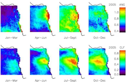
The biomass burning season, from July to September, is characterized by the presence of absorbing particles (probably smoke), with ANG values larger than 1 (Fig. 3). During this time period, aerosol is mostly located above cloud top (60–100 % of cases), as 20

(11)

ACPD

13, 23295–23324, 2013

Title Page

Tables Figures

◭ ◮

Back Close

Full Screen / Esc

Discussion

P

a

per

|

Dis

cussion

P

a

per

|

Discussion

P

a

per

|

Discussio

n

P

a

per

|

cases) and, to a lesser extent, during April–June. If we consider the whole dataset (970 900 retrievals) cases of mixed cloud-aerosol layers account for 34 % (330 988), cases of aerosol above cloud top are 58 % (564 288) and cases of aerosol below cloud base only the remaining 8 % (75 624). In conclusion, the highest spatial and tempo-ral occurrence of mixed case condition is coincident with the most elevated values of 5

Angstrom exponent, giving rise to favourable conditions for positive radiative forcing occurrence during July–September and, to a lesser extent, during October–December.

3.2 All-sky aerosol direct radiative forcing over S-E Atlantic

The all-sky aerosol DRF at TOA is defined as net irradiance in W m−2 between up-welling irradiance computed with a given aerosol load (I_a) and without it (I0) in case 10

of clear and cloudy-sky, weighted by clear-sky (CLF) and cloudy-sky (1-CLF) fraction, respectively. It is calculated as

DRFall=DRFclear+DRFcloudy=I₀clear−I_aclear

(1−CLF)+I₀cloudy−I_acloudy

CLF (6)

According to Eq. (6), all-sky aerosol direct radiative forcing is estimated as the sum of the clear-sky DRF fraction (weighted by clear sky fraction) plus the cloudy-sky DRF 15

fraction (weighted by cloud cover).

Seasonally averaged maps of clear-sky, cloudy-sky DRF and the resulting all-sky estimate are shown in Fig. 2. Maps of Angstrom coefficient and cloud cover are also reported (Fig. 3), to stress the correlation with the associated forcing.

During January–March time-period, the clear-sky DRF (weighted by clear-sky frac-20

tion) is always negative and equal in average to−5.2 W m−2, while locally TOA forc-ing may reach −24.6 W m−2(e.g., over the Gulf of Guinea, in correspondence of the largest values of AOD and ANG). In the same period, cloudy-sky forcing is moder-ately low and equal to 0.3 W m−2, with spatial variations ranging between −1.3 and +4.3 W m−2. This is probably due to the presence of weakly absorbing particles, mostly 25

(12)

ACPD

13, 23295–23324, 2013

Title Page

Tables Figures

◭ ◮

Back Close

Full Screen / Esc

Discussion

P

a

per

|

Dis

cussion

P

a

per

|

Discussion

P

a

per

|

Discussio

n

P

a

per

|

and equal to−4.9 W m−2(Fig. 2). The presence of cloud mitigates the cooling effect of aerosol. The magnitude of the negative forcing is decreased by about 2 W m−2, from the completely clear-sky (assuming CLF₌0, DRF₌−6.9 W m−2) to the all-sky case (CLF=0.26, DRF=−4.9 W m−2).

During April–June, cloud coverage is larger than during the previous trimester. Sim-5

ilarly, AOD (not shown) and ANG values o_ffthe coast of Namibia (where mixed cases of cloud and aerosol layers more frequently occur) are larger. These conditions are favourable to an increase in cloudy-sky forcing and a decrease in clear-sky one. The resulting all-sky DRF is still negative but much smaller, in magnitude, than for January– March (−1.0 W m−2). Cloud presence induces a sensible decrease in the DRF by about 10

4.3 W m−2, from the completely clear-sky (assuming CLF=0, DRF=−5.3 W m−2) to the all-sky case (CLF₌0.36, DRF₌−1.0 W m−2).

Starting from June, the presence of high absorbing aerosol (ANG≥1) mostly located above the cloud top (60–100 % of cases) of extended cloud fields (0.4<CLF<0.9) induces a large positive cloudy-sky (weighted by the cloud cover) DRF, with spatial 15

average equal to+8.8 W m−2. The clear-sky DRF (weighted by the clear sky fraction) is relatively small (−3.5 W m−2). Cloud presence induces an absolute DRF variation of 12.6 W m−2, from the completely clear-sky (assuming CLF=0, DRF=−6.9 W m−2) to the all-sky case (CLF=0.49, DRF= +5.7 W m−2, with local peak up to+46.9 W m−2).

During October–December aerosol load, as well as the Angstrom exponent, de-20

creases substantially back to typical values observed during April–June. However, a higher occurrence of unmixed cases (with aerosol layers above cloud deck) and a larger cloud fraction, with respect to April–June, leads to a small but positive all-sky DRF effect, equal to+0.6 W m−2. This result stresses the critical role of aerosol and clouds mutual position and, hence, of local meteorological conditions on the at-25

(13)

in-ACPD

13, 23295–23324, 2013

Title Page

Tables Figures

◭ ◮

Back Close

Full Screen / Esc

Discussion

P

a

per

|

Dis

cussion

P

a

per

|

Discussion

P

a

per

|

Discussio

n

P

a

per

|

crease equal to 5.8 W m−2, from the clear-sky (assuming CLF=0, DRF=−5.2 W m−2) to the all-sky case (CLF=0.48, DRF= +0.6 W m−2).

When comparing these results with all-sky DRF estimates of Table 1, one must ac-count for the fact that several previous studies only consider the fine-mode fraction of the AOD, because the fine mode fraction is assumed to be of anthropogenic origin. In 5

the present analysis, our aim is to quantify the radiative impact of all (fine and coarse, natural and anthropogenic) species. This approach necessary leads to a significant difference between our results and those reported in Table 1, since aerosol forcing is firstly a function of AOD. The di_fference (all aerosol vs fine mode fraction only) is prob-ably larger when comparing cloudy-sky estimates than for clear-sky. This is because 10

the inclusion of clouds in model simulations results in a stronger TOA forcing sensitiv-ity to aerosol optical properties, as multiple scattering processes between aerosol and clouds get involved.

These considerations may partly explain the large discrepancy with the result of Abel et al. (2005). They find a clear-sky forcing equal to−7.6 W m−2, which is consis-15

tent with our estimation, but a negative spatial average also for the all-sky forcing (for fine aerosol, during September 2000), equal to−3.1 W m−2. For September 2005, we find an all-sky DRF of+9.4±0.8 W m−2(the standard deviation expresses the spatial variability).

Myhre et al. (2003), accounting for AOD from all aerosol species and assuming 20

a constant SSA of 0.90, also find a negative aerosol forcing of −1.7 W m−2 dur-ing September 2000, but smaller than Abel et al. (2005). On the other hand, Keil et al. (2003) obtain very strong and positive all-sky DRF, increasing from 7.5 to 16.9 W m−2as the SSA (assumed constant over the whole area) decreases from 0.93 to 0.85. Their results are coherent with those calculated here, for September 2005, when 25

(14)

ACPD

13, 23295–23324, 2013

Title Page

Tables Figures

◭ ◮

Back Close

Full Screen / Esc

Discussion

P

a

per

|

Dis

cussion

P

a

per

|

Discussion

P

a

per

|

Discussio

n

P

a

per

|

As previously stressed, a large source of error comes from the uncertainties related to vertical profile of cloud and aerosol layers. It is then not surprising that our estimate is significantly different than those obtained from studies that use limited information on temporal distribution of cloud and aerosol layer position (as the two days aircraft campaigns, in the case of the SAFARI experiment).

5

CALIPSO may be a key instrument to assess aerosol direct (and indirect) forcing, as suggested by recent works of Chand et al. (2009) and Sakaeda et al. (2011). The methodology they used to detect aerosol in elevated atmospheric layers above cloud decks, however, differs from our method in several aspects. They assume that aerosol properties retrieved along a single CALIPSO pass are fully representative of 10

local aerosol position, within a 5◦×5◦grid box. In this work, we calculate the mean sea-sonal position of aerosol and cloud at 1◦ resolution, averaging CALIPSO observations collected from 2006 to 2010. Uncertainties coming from both assumptions have not yet been tested and may lead to di_fferent errors in DRF estimates.

Although, Chand et al. (2009) do not provide an overall spatial mean of the 15

all-sky DRF, their estimates varies spatially between −2 and +14 W m−2, during the July–October time period of 2006 and 2007. Even if much smaller in mag-nitude, this is consistent with present calculations, where all-sky DRF is equal to +6.4 [−5.3 to +55.1] W m−2(during July–October, 2006), and equal to +7.2 [−6.7 to +56.9] W m−2(during July–October, 2007). The discrepancy with Chand et al. (2009) 20

may be due to the fact that they consider only AOD from aerosol layers located above the cloud top. As a consequence, aerosol optical thickness is reduced and DRF results weaker (note also that CALIPSO aerosol optical depth is sensibly smaller than that re-trieved by MODIS). In addition, we obtain positive forcing also in case of cloud-aerosol mixing. Neglecting the contribution of mixed layers may lead to substantial underesti-25

(15)

ACPD

13, 23295–23324, 2013

Title Page

Tables Figures

◭ ◮

Back Close

Full Screen / Esc

Discussion

P

a

per

|

Dis

cussion

P

a

per

|

Discussion

P

a

per

|

Discussio

n

P

a

per

|

As a consequence, they neglect cases of high negative forcing due to largely reflecting aerosol, as well as high positive forcing due to largely absorbing aerosol above optically thick clouds.

Sakaeda et al. (2011) calculate monthly averages of all-sky DRF, from carbona-ceous aerosol alone. During the July–October time period, from 2001 to 2008, they 5

find a mean value equal to+1.2 W m−2. This is about six times lower than that calcu-lated in this work, during July–October from 2005 to 2010, equal to+6.8 W m−2. In they simulations, aerosol load is obtained from CALIPSO observations, while the fine-mode fraction is from MODIS monthly product at 5◦resolution. Again, the smaller DRF value found by Sakaeda et al. (2011) can be explained by the choice of using CALIPSO 10

instead of MODIS AOD.

Model simulations of all-sky DRF for 2006–2010 (summarized in Table 2) exhibit a strong and well defined annual cycle, similar to that of 2005, characterized by lim-ited inter-annual variability with respect to seasonal variations. Especially during the biomass burning season, but also during January–March, large spatial standard devi-15

ations indicate strong geographical variability of DRF, during all years.

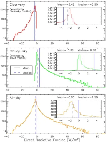
Considering the full time window, from 2005 to 2010, it is possible to quantify the overall all-sky aerosol forcing at TOA over the South-East Atlantic, analysing the clear-sky and cloudy-clear-sky components separately (Fig. 4).

The clear-sky DRF (weighted by clear sky fraction) shows a global mean value of 20

−3.42 W m−2 and a relatively small spatial standard deviation equal to +2.81 W m−2, which indicates a certain geographical homogeneity. The spatial mean of cloudy-sky fraction of DRF is in turn positive and equal to +3.39 W m−2. Its standard deviation is much larger than in case of clear-sky and equal to 7.41 W m−2, showing that cloud cover strongly modulates aerosol forcing. The six year averages of all-sky DRF is close 25

(16)

ACPD

13, 23295–23324, 2013

Title Page

Tables Figures

◭ ◮

Back Close

Full Screen / Esc

Discussion

P

a

per

|

Dis

cussion

P

a

per

|

Discussion

P

a

per

|

Discussio

n

P

a

per

|

Assuming completely cloud-free grid box, the mean value of clear-sky DRF results equal to −4.50 W m2, while the median value is −5.72 W m−2. This is very similar to global satellite-based clear-sky DRF estimates for natural plus anthropogenic aerosols over ocean of 5.5 W m−2(Yu et al., 2006) and 5.0 W m−2(Chen et al., 2008).

3.3 All-sky DRE dependence on CLF

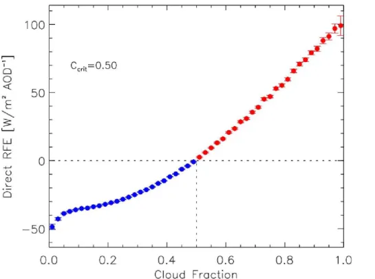
5

Recent studies (Chan et al., 2009; Sakaeda et al., 2011) have confirmed that cloud fraction plays a major role in determining whether DRF at TOA is positive or negative. This is also clearly demonstrated in Fig. 5, that shows the positive co-variation be-tween cloud coverage and aerosol all-sky Direct Radiative Efficiency (DRE). The latter parameter is defined as the DRF per unit of AOD forcing. In Fig. 5, DRE estimates 10

are averaged over constant bin of CLF of 0.2. Aerosol forcing efficiency increases from approximately−50 W m−2 to very high positive values up to 100 W m−2, as CLF varies from almost 0 (clear sky) to 1 (overcast condition). Error bars represent the confidence level of the mean values if one assumes independent data. They are calculated as σ(n−2)−1/2, where nis the number of DRF measurements within the bin andσtheir 15

standard deviation.

It is possible to identify a critical cloud fraction, CLFcrt, beyond which DRE becomes positive. Recent estimates of CLF_crt ranges between 0.4 and 0.5 (Chan et al., 2009; Sakaeda et al., 2011). In particular, Chan et al. (2009) find a clear linear DRE-CLF relationship and a CLFcrtof 0.4, considering only aerosol particles with a constant SSA 20

(at 50 nm) equal to of 0.85, with an associated uncertainty of 0.02, located above cloud deck. In the attempt to provide a more general relationship, we consider all aerosol species (i.e., ANG varies between 0 and 1.5) and all aerosol layer position with respect to cloud filed (mixed, under and above). The resulting CLF-DRE relationship (Fig. 5) clearly shows a CLFcrt equal to 0.5. This observation confirms that CLF is an essen-25

(17)

ACPD

13, 23295–23324, 2013

Title Page

Tables Figures

◭ ◮

Back Close

Full Screen / Esc

Discussion

P

a

per

|

Dis

cussion

P

a

per

|

Discussion

P

a

per

|

Discussio

n

P

a

per

|

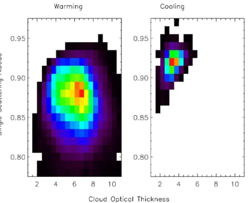
3.4 Cloudy-sky DRF dependence on SSA and COT

This multi-year study of DRF allows us to perform a statistical analysis of the four stream approximation solutions, for SSA and COT. To this purpose, we only consider cloud-sky DRF estimates, in the specific case of aerosol located above the cloud layer. Figure 6 shows two histograms of SSA and COT for positive (left image) and negative 5

(right image) forcing. Colour scale represents arbitrary units, proportional to the number of points within each bin (black/blue indicates few measurements, yellow/red indicates numerous measurements). For a total of 53 549 points, the great majority of cases (96 %) shows positive forcing, mostly characterized by particles with SSA<0.91 and clouds with COT>4 (with typical SSA and COT values of about 0.88 and 7.0). As for 10

critical cloud fraction, SSA=0.90 and COT=4 can be considered as typical threshold values to predict the sign of DRF over the oceans, within [4◦N–30◦S]. On the other hand, the occurrence of negative forcing needs the presence of more reflecting aerosol particles, with SSA>0.91, and optically thin clouds with COT<4 (or no clouds).

4 Discussion

15

Among the several uncertainties and error sources that come from the different hypoth-esis made in this work and described in previous sections, we stress that the aerosol and cloud diurnal cycles have been neglected for lack of suitable information. The opti-cal and spatial properties of both aerosols and clouds are obtained from daily product derived from instantaneous satellite overpass. Further analysis is needed to analyse 20

(18)

ACPD

13, 23295–23324, 2013

Title Page

Tables Figures

◭ ◮

Back Close

Full Screen / Esc

Discussion

P

a

per

|

Dis

cussion

P

a

per

|

Discussion

P

a

per

|

Discussio

n

P

a

per

|

provide higher temporal resolution than with the two MODIS instrument observations (per daytime), geostationary satellite (e.g., Meteosat-8) observations shall be used.

Another source of error that may sensible affect DRF estimates is the variation of the aerosol radiative effect with the SZA. In this work, we only consider the daily mean cosine of SZA, to account for the average sun inclination for each day. Some studies 5

suggest that an adequate time step should be dramatically smaller, less than 30 min (Yu et al., 2004), in order to sample DRF from a wide range of solar zenith angles. Although more accurate, we did not use this approach because of its computational cost. However, the South-East Atlantic region is mostly characterized by the presence of highly absorbing aerosol and the relative radiative effect is supposed to have a rela-10

tively small SZA dependence (Yu et al., 2002).

5 Summary and conclusions

In this work, we attempt a more accurate estimate of aerosol DRF using a shortwave radiative transfer model constrained by satellite observations of aerosols and cloud parameters, including their vertical positioning, and a parametrisation of the aerosol 15

absorption. The satellite observations are based on statistical analysis of both MODIS and CALIPSO products over the South-East Atlantic.

Model simulations for the whole 2005–2010 time period indicate that monthly DRF averages show a strong annual cycle, with mean value and spatial standard deviation of about −4.3±4.3 (January–March), −2.1±2.1 (April–June), +5.6±10.5 20

(July–September) and +0.6±3.4 W m−2 (October–December). The inter-annual vari-ability is small with respect to seasonal variations. During the six year time period, the mean aerosol direct e_ffect is averaged over the whole region is almost zero (−0.03±8.14 W m−2), indicating a near perfect compensation between the clear-sky (−3.42±2.81 W m−2) and the cloudy-sky (3.39±7.41 W m−2) forcings. Although the 25

(19)

ACPD

13, 23295–23324, 2013

Title Page

Tables Figures

◭ ◮

Back Close

Full Screen / Esc

Discussion

P

a

per

|

Dis

cussion

P

a

per

|

Discussion

P

a

per

|

Discussio

n

P

a

per

|

(−0.5 W m−2) in the International Intergovernmental Panel Climate Change report (Fos-ter et al., 2007), which is a consequence of the much larger absorption than the “typi-cal” aerosol. The large spatial standard deviation, however, indicates that locally (with a 1◦×1◦grid box) the monthly averaged DRF can be much larger in magnitude, either positive or negative. In conclusion, over South-East Atlantic, cooling and warming ef-5

fects are somewhat balanced. This is mostly due to the occurrence of large amounts of smoke particles during the biomass burning season. Therefore, other oceanic re-gions characterized by lower occurrence of absorbing particles are expected to pro-duce much stronger cooling at TOA.

It has been also shown that CLF is as a good predictor of direct forcing efficiency. In 10

particular a CLF of 0.5 can be considered as the threshold value beyond which all-sky TOA forcing becomes positive. At the same time, we find that positive cloudy-sky DRF mostly occurs in case of aerosol particles with single scattering albedo smaller than 0.91 above cloud with optical thickness larger than 4.

The strong hypotheses made in this work primary concern the parametrization of 15

aerosol optical properties (in particular on SSA, parametrized from ANG satellite ob-servation), their diurnal cycle (not considered), aerosol layer altitudes (defined with respect to cloud altitude and placed at a fixed distance from cloud layer) and solar zenith angle (only daily averages are considered). They have permitted to obtain DRF estimates, considering a wide range of parameters that are usually neglected in previ-20

ous studies (e.g., the temporal and spatial variability of SSA and aerosol-cloud vertical distribution), with a reasonably small computational effort. However, further work is needed to analyse the DRF sensitivity to such hypotheses.

Nevertheless, this work remains of particular interest as the quantification of aerosol DRF (and IRF) over different Earth’s regions is a fundamental issue for climate studies. 25

(20)

ACPD

13, 23295–23324, 2013

Title Page

Tables Figures

◭ ◮

Back Close

Full Screen / Esc

Discussion

P

a

per

|

Dis

cussion

P

a

per

|

Discussion

P

a

per

|

Discussio

n

P

a

per

|

that is still poorly quantified.

The publication of this article is financed by CNRS-INSU.

References

Abel, S. J., Highwood, E. J., Haywood, J. M., and Stringer, M. A.: The direct radiative ef-5

fect of biomass burning aerosols over southern Africa, Atmos. Chem. Phys., 5, 1999–2018, doi:10.5194/acp-5-1999-2005, 2005.

Br ´eon F. M. and Doutriaux-Boucher, M.: A comparison of cloud droplet radii measured from space, IEEE Trans Geosc. Rem. Sens., 43, 1796–1805, 2005.

Chand, D., Wood, R., Anderson, T. L., Satheesh, S. K., and Charlson, R. J.: Satellite-derived 10

direct radiative effect of aerosols dependent on cloud cover, Nat. Geosci., 2, 181–184, doi:10.1038/ngeo437, 2009.

Charlson, R. J., Langer, J., Rodhe, H., Leovy, C. B., and Warren, S. G.: Perturbation of the Northern Hemisphere radiative balance by backscattering from anthropogenic aerosols, Tel-lus, 43, 152–163, 1991.

15

Charlson, R. J., Schwartz, S. E., Hales, J. M., Cess, R. D., Coakley Jr., J. A., Hansen, J. E., and Hofmann, D. J.: Climate forcing by anthropogenic aerosols, Science, 255, 423–430, 1992. Chen, Lin, Shi, Guang-Yu, and Zhong, Ling-Zhi: Short-Wave Direct Radiative Effect of Aerosols

in the Clear-Sky over Oceans from Satellites Observations, ettandgrs, vol. 1, 567–570, 2008 International Workshop on Education Technology and Training & 2008 International Work-20

shop on Geoscience and Remote Sensing, 2008.

Chylek, P. and Wong, J.: Effect of absorbing aerosols on global radiation budget, Geophys. Res. Lett., 22, 929–931, 1995.

Costantino, L. and Br ´eon, F.-M.: Analysis of aerosol-cloud interaction from multi-sensor satellite observations, Geophys. Res. Lett., 37, L11801, doi:10.1029/2009GL041828, 2010.

(21)

ACPD

13, 23295–23324, 2013

Title Page

Tables Figures

◭ ◮

Back Close

Full Screen / Esc

Discussion

P

a

per

|

Dis

cussion

P

a

per

|

Discussion

P

a

per

|

Discussio

n

P

a

per

|

Costantino, L. and Br ´eon, F.-M.: Aerosol indirect effect on warm clouds over South-East At-lantic, from co-located MODIS and CALIPSO observations, Atmos. Chem. Phys., 13, 69–88, doi:10.5194/acp-13-69-2013, 2013.

Dubovik, O., Holben, B. N., Eck, T. F., Smirnov, A., Kaufman, Y. J., Kin, G. M. D., Tanr `ı, D., and Slutsker, I.: Variability of absorption and optical properties of key aerosol types observed in 5

worldwide locations, J. Atmos. Sci., 59, 590–608, 2002.

Feingold, G., Eberhard, W. L., Veron, D. E., and Previdi, M.: First measurements of the Twomey indirect effect using ground-based remote sensors, Geophys. Res. Lett., 30, 1287, doi:10.1029/2002GL016633, 2003.

Forster, P., Ramaswamy, V., Artaxo, P., Berntsen, T., Betts, R., Fahey, D. W., Haywood, J., 10

Lean, J., Lowe, D. C., Myhre, G., Nganga, J., Prinn, R., Raga, G., M. Schulz and Van Dor-land, R.: Changes in atmospheric constituents and in radiative forcing, in: Climate Change 2007: The Physical Science Basis, Contribution of Working Group I to the Fourth Assess-ment Report of the IntergovernAssess-mental Panel on Climate Change, edited by: Solomon, S., Qin, D., Manning, M., Chen, Z., Marquis, M., Averyt, K. B., Tignor, M., and Miller, H. L., 15

Cambridge University Press, Cambridge, UK and New York, NY, USA, 2007.

Garay, M. J., de Szoeke, S. P., and Moroney, C. M.: Comparison of marine stratocumulus cloud top heights in the southeastern Pacific retrieved from satellites with coincident ship-based observations, J. Geophys. Res., 113, D18204, doi:10.1029/2008JD009975, 2008.

Harshvardhan, Zhao, G., Di Girolamo, L., and Green, R. N.: Satellite-observed location of stra-20

tocumulus cloudtop heights in the presence of strong inversions, IEEE T. Geosci. Remote S., 47, 1421–1428, doi:10.1109/TGRS.2008.2005406, 2009.

Hatzianastassiou, N., Matsoukas, C., Drakakis, E., Stackhouse Jr., P. W., Koepke, P., Fotiadi, A., Pavlakis, K. G., and Vardavas, I.: The direct effect of aerosols on solar radiation based on satellite observations, reanalysis datasets, and spectral aerosol optical properties from 25

Global Aerosol Data Set (GADS), Atmos. Chem. Phys., 7, 2585–2599, doi:10.5194/acp-7-2585-2007, 2007.

Haywood, J. and Shine, K.: The effect of anthropogenic sulfate and soot aerosol on the clear sky planetary radiation budget, Geophys. Res. Lett., 22, 603–606, 1995.

Ichoku, C., Remer, L. A., Kaufman, Y. J., Levy, R., Chu, D. A., Tanr ´e, D., and Hol-30

(22)

ACPD

13, 23295–23324, 2013

Title Page

Tables Figures

◭ ◮

Back Close

Full Screen / Esc

Discussion

P

a

per

|

Dis

cussion

P

a

per

|

Discussion

P

a

per

|

Discussio

n

P

a

per

|

Johnson, B. T., Osborne, S. R., Haywood, J. M., and Harrison, M. A. J.: Aircraft measure-ments of biomass burning aerosols over West Africa during DABEX, J. Geophys. Res., 113, D00C06, doi:10.1029/2007JD009451, 2008.

Keil, A. and Haywood, J. M.: Solar radiative forcing by biomass burning aerosol particles during SAFARI 2000: a case study based on measured aerosol and cloud properties, J. Geophys. 5

Res., 108, 8467, doi:10.1029/2002JD002315, 2003.

McComiskey, A., Schwartz, S. E., Schmid, B., Guan, H., Lewis, E. R., Ricchiazzi, P., and Ogren, J. A.: Direct aerosol forcing: calculation from observables and sensitivities to inputs, J. Geophys. Res., 113, D09202, doi:10.1029/2007JD009170, 2008.

McConnell, C. L., Highwood, E. J., Coe, H., Formenti, P., Anderson, B., Osborne, S., Nava, S., 10

Desboeufs, K., Chen, G., and Harrison, M. A. J.: Seasonal variations of the physical and optical characteristics of Saharan dust: results from the Dust Outflow and Deposition to the Ocean (DODO) experiment, J. Geophys. Res., 113, D14S05, doi:10.1029/2007JD009606, 2008.

Menzel, W. P., Frey, R. A., Zhang, H., Wylie, D. P., Moeller, C. C., Holz, R. E., Maddux, B, 15

Baum, B. A., Strabala, K. I., Gumley, L. E.: MODIS global cloud-top pressure and amount estimation: algorithm description and results, J. Appl. Meteorol. Climatol., 47, 1175–1198, 2008.

Myhre, G., Berntsen, T. K., Haywood, J. M., Sundet, J. K., Holben, B. N., Johnsrud, M., and Stordal, F.: Modelling the solar radiative impact of aerosols from biomass burning during the 20

Southern African Regional Science Initiative (SAFARI-2000) experiment, J. Geophys. Res., 108, 8501, doi:10.1029/2002JD002313, 2003.

Nemesure, S., Wagener, R., and Schwartz, S. E.: Direct shortwave forcing of climate by an-thropogenic sulfate aerosol: sensitivity to particle size, composition, and relative humidity, J. Geophys. Res., 100, 26105–26116, 1995.

25

Osborne, S. R., Johnson, B. T., Haywood, J. M., Baran, A. J., Harrison, M. A. J., and Mc-Connell, C. L.: Physical and optical properties of mineral dust aerosol during the dust and biomass-burning experiment, J. Geophys. Res., 113, D00C03, doi:10.1029/2007JD009551, 2008.

Penner, J., Dickinson, R., and O’Neill, C.: Effects of aerosol from biomass burning on the global 30

(23)

ACPD

13, 23295–23324, 2013

Title Page

Tables Figures

◭ ◮

Back Close

Full Screen / Esc

Discussion

P

a

per

|

Dis

cussion

P

a

per

|

Discussion

P

a

per

|

Discussio

n

P

a

per

|

Queface, A. J., Piketh, S. J., Annegarn, H. J., Holben, B. N., Uthui, R. J.: Retrieval of aerosol optical thickness and size distribution from the CIMEL sun photometer over Inhaca island, Mozambique, J. Geophys. Res., 108, 8509, doi:10.1029/2002JD002374, 2003.

Sakaeda, N., Wood, R., and Rasch, P. J.: Direct and semidirect aerosol effects of southern African biomass burning aerosol, J. Geophys. Res., 116, D12205, 5

doi:10.1029/2010JD015540, 2011.

Smirnov A, Holben, B. N., Kaufman, Y. J., Dubovik O, Eck, T. F., Slutsker I, Pietras C, Halthore, R. N.: Optical properties of atmospheric aerosol in maritime environments, J. At-mos. Sci., 59, 501–523, 2002.

Stamnes, K., Tsay, S.-C., Wiscombe, W., and Jayaweera, K.: Numerically stable algorithm for 10

discrete-ordinate-method radiative transfer in multiple scattering and emitting layered media, Appl. Optics, 27, 2502–2509, 1988.

Thieuleux, F., Moulin, C., Br ´eon, F. M., Maignan, F., Poitou, J., and Tanr ´e, D.: Remote sensing of aerosols over the oceans using MSG/SEVIRI imagery, Ann. Geophys., 23, 3561–3568, doi:10.5194/angeo-23-3561-2005, 2005.

15

Yu, H., Liu, S. C., and Dickinson, R. E.: Radiative effects of aerosols on the evolution of the at-mospheric boundary layer, J. Geophys. Res., 107, 4142, doi:10.1029/2001JD000754, 2002. Yu, H., Dickinson, R. E., Chin, M., Kaufman, Y. J., Zhou, M., Zhou, L., Tian, Y., Dubovik, O.,

and Holben, B. N.: The direct radiative effect of aerosols as determined from a combi-nation of MODIS retrievals and GOCART simulations, J. Geophys. Res., 109, D03206, 20

doi:10.1029/2003JD003914, 2004.

Yu, H., Quinn, P. K., Feingold, G., Remer, L. A., Kahn, R. A., Chin, M., and Schwartz, S. E.: Remote sensing and in situ measurements of aerosol properties, burdens, and radiative forc-ing, in: Atmospheric Aerosol Properties and Climate Impacts, A Report by the US Climate Change Science Program and the Subcommittee on Global Change Research, edited by: 25

(24)

ACPD

13, 23295–23324, 2013

Title Page

Tables Figures

◭ ◮

Back Close

Full Screen / Esc

Discussion

P

a

per

|

Dis

cussion

P

a

per

|

Discussion

P

a

per

|

Discussio

n

P

a

per

|

Table 1.Recent estimates of all-sky aerosol (fine and coarse mode if not specified) shortwave

direct radiative forcing at TOA, over South-East Atlantic, from model simulations constrained by satellite data. Minimum and maximum values are reported, if present, within the square brackets.

Global DRF over South-Est Atlantic [W m−2_] _Remarks

Sakaeda et al. (2011) _2.3

Forcing weighted by cloudy-sky fraction

Jul–Oct, 2001–2008 Carbonaceous aerosol

Chand et al. (2009) [−2, 14] Jul–Oct, 2006–2007_SSA

=0.85 Hatzianastassiou et al.

(2007) −1.62 [−15, 10]

Whole planet (ocean and land) Jan–Jul, 1984–1993

Abel et al. (2005) −3.1 [−13.1, 5.1] Sep, 2000 (SAFARI)_{Fine aerosol}

Myhre et al. (2003)

−1.7 [−20, 6] Sep, 2000 (SAFARI)_SSA

=0.90 [−50, 65]

Instantaneous DRF

5–19 Sep, 2000, at 09:00 UTC SSA=0.90

Ichoku et al. (2003) −10 Sep, 2000 (SAFARI)_SSA₌_0.90 Keil et al. (2003) SSA=0.93 SSA=0.90 SSA=0.85 7 Sep, 2000 (SAFARI)

(25)

ACPD

13, 23295–23324, 2013

Title Page

Tables Figures

◭ ◮

Back Close

Full Screen / Esc

Discussion

P

a

per

|

Dis

cussion

P

a

per

|

Discussion

P

a

per

|

Discussio

n

P

a

per

|

Fig. 1.Frequency of occurrence (from 0 and 1) of cases with aerosol layers mixed, unmixed

(26)

ACPD

13, 23295–23324, 2013

Title Page

Tables Figures

◭ ◮

Back Close

Full Screen / Esc

Discussion

P

a

per

|

Dis

cussion

P

a

per

|

Discussion

P

a

per

|

Discussio

n

P

a

per

|

Fig. 2.Shortwave clear-sky DRF, weighted by clear-sky fraction (top image), cloudy-sky DRF,

(27)

ACPD

13, 23295–23324, 2013

Title Page

Tables Figures

◭ ◮

Back Close

Full Screen / Esc

Discussion

P

a

per

|

Dis

cussion

P

a

per

|

Discussion

P

a

per

|

Discussio

n

P

a

per

|

Fig. 3.Seasonal maps of Angstrom coefficient (top image) and cloud fraction (bottom image),

(28)

ACPD

13, 23295–23324, 2013

Title Page

Tables Figures

◭ ◮

Back Close

Full Screen / Esc

Discussion

P

a

per

|

Dis

cussion

P

a

per

|

Discussion

P

a

per

|

Discussio

n

P

a

per

|

Fig. 4.Histograms of 1◦×1◦model estimates of clear-sky fraction (top image), cloud-sky

(29)

ACPD

13, 23295–23324, 2013

Title Page

Tables Figures

◭ ◮

Back Close

Full Screen / Esc

Discussion

P

a

per

|

Dis

cussion

P

a

per

|

Discussion

P

a

per

|

Discussio

n

P

a

per

|

Fig. 5.DRE at TOA as a function of cloud fraction.C_crit is the critical cloud fraction for which

(30)

ACPD

13, 23295–23324, 2013

Title Page

Tables Figures

◭ ◮

Back Close

Full Screen / Esc

Discussion

P

a

per

|

Dis

cussion

P

a

per

|

Discussion

P

a

per

|

Discussio

n

P

a

per

|

Fig. 6.Number concentration of SSA and COT retrievals, from MODIS daily product in case of