www.atmos-chem-phys.net/11/11951/2011/ doi:10.5194/acp-11-11951-2011
© Author(s) 2011. CC Attribution 3.0 License.
Chemistry
and Physics
Assessing regional scale predictions of aerosols, marine
stratocumulus, and their interactions during VOCALS-REx
using WRF-Chem
Q. Yang1, W. I. Gustafson Jr.1, J. D. Fast1, H. Wang1, R. C. Easter1, H. Morrison2, Y.-N. Lee3, E. G. Chapman1, S. N. Spak4, and M. A. Mena-Carrasco5
1Pacific Northwest National Laboratory, Richland, WA, USA 2National Center for Atmospheric Research, Boulder, CO, USA 3Brookhaven National Laboratory, Upton, New York, USA 4Public Policy Center, University of Iowa, Iowa City, IA, USA
5Center for Sustainability Research, Universidad Andr´es Bello, Santiago, Chile Received: 22 July 2011 – Published in Atmos. Chem. Phys. Discuss.: 11 August 2011 Revised: 3 November 2011 – Accepted: 8 November 2011 – Published: 2 December 2011
Abstract.This study assesses the ability of the recent chem-istry version (v3.3) of the Weather Research and Forecast-ing (WRF-Chem) model to simulate boundary layer struc-ture, aerosols, stratocumulus clouds, and energy fluxes over the Southeast Pacific Ocean. Measurements from the VA-MOS Ocean-Cloud-Atmosphere-Land Study Regional Ex-periment (VOCALS-REx) and satellite retrievals (i.e., prod-ucts from the MODerate resolution Imaging Spectrora-diometer (MODIS), Clouds and Earth’s Radiant Energy Sys-tem (CERES), and GOES-10) are used for this assessment. The Morrison double-moment microphysics scheme is newly coupled with interactive aerosols in the model. The 31-day (15 October–16 November 2008) WRF-Chem simula-tion with aerosol-cloud interacsimula-tions (AERO hereafter) is also compared to a simulation (MET hereafter) with fixed cloud droplet number concentrations in the microphysics scheme and simplified cloud and aerosol treatments in the radiation scheme. The well-simulated aerosol quantities (aerosol num-ber, mass composition and optical properties), and the inclu-sion of full aerosol-cloud couplings lead to significant im-provements in many features of the simulated stratocumulus clouds: cloud optical properties and microphysical proper-ties such as cloud top effective radius, cloud water path, and cloud optical thickness. In addition to accounting for the aerosol direct and semi-direct effects, these improvements feed back to the simulation of boundary-layer characteris-tics and energy budgets. Particularly, inclusion of
interac-Correspondence to:Q. Yang (qing.yang@pnnl.gov)
1 Introduction
Marine stratocumuli play an important role in radiation and hydrological budgets, particularly along the eastern edges of oceans, such as over the Southeast Pacific Ocean (SEP) (Stevens et al., 2005; Stevens and Feingold, 2009). These clouds are bright compared to the dark ocean surface and result in much more shortwave radiation scattered back to space. Their effective temperature is comparable to that of the ocean surface, so the emitted longwave radiation im-poses little compensating effect. Therefore, properly repre-senting these clouds in climate models is important. How-ever, marine stratocumuli are notoriously difficult to model accurately. The recent Preliminary VOCALS model As-sessment (PreVOCA) (Wyant et al., 2010) showed a wide range in behavior among models in representing such clouds. One reason for this difference is the simplified treatments of aerosols used by most models, for example, assuming a constant background aerosol concentration or cloud droplet number concentration in the microphysics modules. In real-ity, strong gradients in aerosol number and composition exist as one progresses westward from the coast towards the open ocean. These gradients result in cloud condensation nuclei (CCN) gradients and lead to differing cloud characteristics as well.
Reproducing CCN gradients and including coupled cloud-aerosol-radiation processes are important to properly sim-ulate the marine stratocumulus over the SEP. This pa-per shows the improvement gained in using an interactive aerosol-cloud-radiation module in the chemistry version of the Weather Research and Forecasting (WRF-Chem) model (Grell et al., 2005; Fast et al., 2006). Specifically, a new cou-pling between the double-moment Morrison microphysics scheme (Morrison et al., 2005, 2009) and the aerosol mod-ules is used; we implemented this coupling in the April 2011 v3.3 release of WRF-Chem. The VAMOS Ocean-Cloud-Atmosphere-Land Study Regional Experiment (VOCALS-REx) was a field campaign during October and November 2008 designed to improve the scientific understanding of model simulations and predictions of the coupled climate system over the SEP (Wood et al., 2011b). The campaign provided extensive measurements for evaluating the capabil-ity of our model with the aforementioned new coupling in predicting aerosol and marine stratus clouds over this region. A recent modeling exercise by Abel et al. (2010) using the UK Met Office Unified Model (MetUM) is parallel to this model evaluation study. MetUM simulated a good rep-resentation of synoptically induced variability in cloud cover and boundary layer depth during the VOCALS-REx (Abel et al., 2010). However, the exclusion of cloud-aerosol interac-tions and the model’s relatively simple parameterization of cloud-microphysical effects (Toniazzo et al., 2011) are likely to preclude better agreement with field observations.
Aerosol-cloud interactions are important to the variability of marine stratus. Aerosols can impact radiative fluxes
di-rectly through absorption and scattering (the direct effect), semi-directly through the impact of aerosol absorption on atmospheric heating and stability (semi-direct effect), and indirectly through their impact on liquid clouds via the so-called indirect effects (Twomey, 1977; Albrecht, 1989). The first indirect effect is the change in cloud albedo due to the change in cloud droplet number and radius. The second in-direct effect (also known as the “cloud lifetime effect”) is the change in cloud lifetime and precipitation due to change in cloud droplet number; the importance of this effect on ra-diative forcing is evident in shallow marine status (Stevens and Feingold, 2009). By changing warm-rain processes in marine stratocumulus clouds, aerosols can alter cloud cellu-lar structures and boundary-layer mesoscale circulations in ways that are much more complicated than traditionally de-picted by conceptual models of the indirect effects (Steven et al., 2005; Wang and Feingold, 2009a, b). The emerging importance and complexity of aerosol-cloud-precipitation in-teractions in shallow marine status is gaining recognition by the scientific community (Stevens and Feingold, 2009). These aerosol-cloud interactions and associated dynamical feedbacks are particularly important over the SEP.
The strong gradients of anthropogenic and natural aerosols in the marine boundary layer (MBL), make the SEP an ideal location for studying the response of shallow marine clouds to aerosol perturbations. Along the coast of Chile and Peru, copper smelters, power plants, and oil refineries emit large amounts of oxidized sulfur (sulfur dioxide (SO2) + sulfate) (Huneeus et al., 2006). Other continental sources include volcanic, biomass burning, biogenic, and dust emissions. As-sociated with mid-latitude synoptic-scale disturbances, east-erly flow subsides down the subtropical Andes, and brings the emitted trace gases and particles over the continent to the stratus deck (Huneeus et al., 2006). These continen-tal pollutants, both primary and secondary, are then mixed with trace gases and particles from oceanic emissions. Ma-rine sources of primary aerosols include sea-salt and organic compounds from sea spray and bubble bursting (Russell et al., 2010), and a source of secondary aerosols is the oxidation of dimethyl sulfide (DMS) to sulfate and methanesulfonic acid (MSA). Detailed understanding of the aerosol-cloud in-teractions (e.g., the transition from closed to open cellular convection) and properly reproducing the climate impact of these clouds remain a challenge for current climate model-ing.
and simplified cloud and aerosol treatments in the radia-tion scheme. A descripradia-tion of the model and observaradia-tional data is provided in Sect. 2. In Sect. 3, we first discuss the characteristics of the simulated marine boundary layer (Sect. 3.1), then evaluate simulated aerosol (Sect. 3.2), cloud optical properties (Sect. 3.3) and cloud macro structures (Sect. 3.4). The domain-average top-of-atmosphere (TOA) shortwave (SW) fluxes and longitudinal and diurnal vari-ations in surface energy fluxes are discussed in Sect. 3.5. Model representations of longitudinal and vertical variations of drizzle are shown in Sect. 3.6. The discussion and sum-mary of the evaluation results are presented in Sects. 4 and 5, respectively.
2 Model description and observational data
2.1 WRF-Chem
WRF-Chem is a widely used regional model employed op-erationally for air quality (e.g., Zhang et al., 2010) and tracer forecasting (http://www-frd.fsl.noaa.gov/aq/wrf/), de-tailed aerosol process studies (e.g., Fast et al., 2009), and regional climate studies involving aerosols (e.g., Qian et al., 2009). It includes full online interactions between aerosols, radiation, and clouds for the direct, semi-direct, and first and second indirect effects as described in Fast et al. (2006), Chapman et al. (2009), and Gustafson et al. (2007). Past re-search included aerosol indirect effects only through the Lin microphysics scheme. This has now been complemented in WRF-Chem v3.3 with the additional option to use the Morri-son microphysics scheme. The simulations presented in this study were performed by using the code as implemented in WRF-Chem v3.2.1, which was then released to the public in v3.3.
For comparison purposes, two simulations were con-ducted: one with aerosol-cloud interactions (referred to as AERO) and the other with aerosol and chemistry modules turned off and droplet number prescribed (referred to as MET). Table 1 shows the model configuration used for the simulations in this study. The configuration is representative for simulations involving full aerosol-climate effects. The Model for Simulating Aerosol Interactions and Chemistry (MOSAIC) (Zaveri et al., 2008) is implemented with a sec-tional approach where the size distributions for both unacti-vated/interstitial and activated aerosols are represented with 8 bins whose lower and upper dry diameters are listed in Ta-ble 2. What is new compared to previous published stud-ies using the MOSAIC aerosol module is the inclusion of DMS chemistry as a source of atmospheric SO2and sulfuric acid (H2SO4). In this study, a correction has been made to the reaction rate for the decomposition of methanesulfonyl (CH3SO2)radicals into SO2, which has been incorporated into WRF-Chem v3.3. Secondary organic aerosol formation (Shrivastava et al., 2010) is not included in the simulations
presented here to reduce the overall computational expense and, as shown later, organic aerosols are a relatively small fraction of the total aerosol mass over the SEP. Subgrid cu-mulus parameterization was turned off for the simulations in this study due to the following reasons. The predomi-nant clouds during VOCALS-REx were marine stratocumu-lus, which are generally not treated well by cumulus param-eterizations. In a short 9-day test run using the Kain-Fritsch cumulus scheme, there was no apparent improvement in sim-ulated cloud features and precipitation. Also, the cumulus schemes currently in WRF-Chem have not been coupled with interactive aerosol.
Table 1.Primary model configuration settings.
Atmospheric Process WRF Option
Tracer advection Monotonic
Longwave radiation RRTM
Shortwave radiation Goddard
Surface layer MM5 similarity theory
Land surface Noah
Boundary layer YSU
Deep and shallow cumulus clouds Turned off
Cloud microphysics Morrison
Gas phase chemistry CBM-Z with DMS reactions
Aerosol chemistry 8-bin MOSAIC (for AERO)
Photolysis Madronich (for AERO)
Aerosol direct & semi-direct effects Turned on (for AERO) Aqueous chemistry, wet scavenging, and cloud-aerosol interactions Turned on (for AERO)
Table 2.Particle dry-diameter range for the eight MOSAIC aerosol size bins employed in this study.
Bin Lower Diameter Upper Diameter
(µm) (µm)
1 0.0390625 0.078125
2 0.078125 0.15625
3 0.15625 0.3125
4 0.3125 0.625
5 0.625 1.25
6 1.25 2.5
7 2.5 5.0
8 5.0 10.0
lifetime. Aerosol effects on longwave radiation are not in-cluded in this study, but have also been recently incorporated into WRF v3.3 as described in Zhao et al. (2010).
Advection of scalar quantities (e.g., aerosol and hydrom-eteor number mixing ratios) was found to be critical to the performance of a double-moment microphysics scheme in-corporated into WRF when simulating stratocumulus clouds with interactive CCN, particularly near strong gradients (Wang et al., 2009); therefore, we employ the monotonic ad-vection scheme for model scalars and chemical species for better accuracy in advection even though it is more compu-tationally expensive.
Simulated evolution of the MBL and stratocumulus clouds will be highly dependent upon the Planetary Boundary Layer (PBL) parameterization with our 9 km horizontal grid spac-ing. In this study, the YSU scheme (Hong et al., 2006) is used, which employs nonlocal-K (vertical diffusion coeffi-cient) mixing for momentum, entrainment of heat and mo-mentum fluxes at the PBL top, a local-K approach for atmo-spheric diffusion above the mixed layer, and a critical bulk Richardson number of zero for the PBL top.
The model domain covers part of the northern Chilean and southern Peruvian coasts and the nearby Southeast Pacific, roughly 63◦W–93◦W in longitude and 11◦S–36◦S in lati-tude. Throughout the paper, two regions, the “coastal region” and the “remote region”, are defined. The two regions are separated by the 78◦W meridian with the west (remote
re-gion) characterized by remote marine aerosol conditions and the east (coastal region) characterized by anthropogenic in-fluences mixed with the maritime background. From the sur-face to 50 hPa, the model has 64 vertical layers, and the layer thickness increases from∼30 m at the surface to ∼50 m at 1 km and∼90 m at 2 km above the ocean surface. The hor-izontal grid spacing is 9 km. Excluding five-days of model spin-up, the simulation period is from 00:00 UTC 15 October 2008 to 00:00 UTC 16 November 2008. Initial conditions, boundary conditions, and time dependent sea surface temper-atures (SSTs) for meteorology were obtained from the Global Forecast System (GFS) model output with a 0.5-degree grid spacing, while the Model for Ozone and Related chemical Tracers (MOZART) provided the initial and boundary con-ditions for trace gases and aerosols. Emissions used for the AERO simulation are as follows. Coarse and fine mode sea-salt emissions are based on Gong et al. (1997) and Mona-han et al. (1986), which neglect sea-salt production through breaking waves, while ultrafine sea-salt emissions follow Clarke et al. (2006). Sea-salt particles are treated as NaCl in the model. DMS emissions are calculated using a sim-plified Nightingale et al. (2000) scheme with constant SST and a geographically uniform ocean surface DMS concentra-tion of 2.8 m mol l−1as specified in the VOCA Modeling Ex-periment Specification (http://www.atmos.washington.edu/
∼mwyant/vocals/model/VOCA Model Spec.htm).
included) and volcanic emissions. Emissions of carbon monoxide (CO), oxides of nitrogen (NOx), SO2, ammo-nia (NH3), black carbon (BC), organic carbon (OC), parti-cles 10 µm or less in diameter (PM10), partiparti-cles 2.5 µm or less in diameter (PM2.5), and volatile organic compounds
(VOCs) are included in the VOCA inventory; oceanic NH3 emissions are not included. Biomass burning emissions (CO, NOx, SO2, NH3, VOCs, OC, BC, and PM2.5) are
based on the MODerate resolution Imaging Spectroradiome-ter (MODIS) fire counts and combustion estimates that de-pend on location-specific vegetation type (Wiedinmyer et al., 2011). Windblown dust emissions are based on the Shaw et al. (2008) formulation.
2.2 Observational data
A wide range of meteorological, trace gas, and aerosol mea-surements were collected during VOCALS-REx as described in Wood et al. (2011b). The NCAR C-130 aircraft and the NOAA Ronald H. Brown research vessel (hereafter RB) were selected as the main measurement platforms for the model evaluation in this study due to two main reasons: (1) both the C-130 and RB provided measurements farther into the remote ocean region (∼88◦W) of the model domain; this extended longitudinal data coverage is necessary for the pur-pose of contrasting different aerosol and cloud characteris-tics over polluted and clean environments; and (2) the RB provided energy fluxes, DMS ocean-to-air transfer velocity, and other near-surface measurements that are important to the model assessment, and those measurements are comple-mentary to measurements obtained on the flight platforms. The selection of the RB as one of the two main platforms leads to the division of the model domain into two regions (remote and costal regions) since the RB sampled more in-tensively around∼85◦W and∼75◦W. Within the domain,
there are about twice as many samples over the coastal re-gion compared to the remote rere-gion from both the C-130 and RB platforms during the VOCALS-REx. Here we briefly de-scribe the observations that are employed in this modeling study. Detailed descriptions of the instruments can be found elsewhere (e.g., Allen et al., 2011; Wood et al., 2011a; Yang et al., 2011).
2.2.1 Aerosol number and mass concentrations
During the VOCALS-REx, a Particle Measurement System (PMS) Passive Cavity Aerosol Spectrometer Probe (PCASP) measured accumulation mode aerosol particles (dry diame-ter 0.117–2.94 µm) on the aircraft. For the purpose of match-ing aerosol particle sizes between PCASP measurements and model simulations, this study uses only measured aerosol particle concentrations with diameters of 0.156–2.69 µm.
Aerosol Mass Spectrometers (AMS) described below measured non-refractory, non-sea-salt mass loading of aerosol sulfate, ammonium, nitrate, and particulate organic
matter (OM). The AMS instruments on the C-130 (De-Carlo et al., 2006) and the United Kingdom (UK) British Aerospace-146 (BAe-146) aircrafts measured aerosol com-ponents aloft for particle sizes (vacuum aerodynamic diam-eter) between 0.05 and 0.5 µm and the AMS on the G-1 air-craft (Kleinman et al., 2011) measured aerosol compositions in the 0.06–0.6 µm diameter range. The AMS (Hawkins et al., 2010) onboard the RB research vessel provided surface-level particle measurements in the submicron range. The BAe-146 AMS dataset retrieved with collection efficiency of 1 was used, and the detailed justification can be found in Allen et al. (2011).
The sub- and supermicron chloride and sodium aerosols were sampled by two-stage multi-jet cascade impactors (CIS) on the RB, with 50 % aerodynamic cutoff diameters of 1.1 and 10 µm at 60 % relative humidity. Submicron chlo-ride and sodium were also sampled by a Particle Into Liquid Sampler (PILS) on the G-1 aircraft, with a sampled particle size range of 0.06–1.5 µm at ambient humidity. The samples obtained with both the CIS and PILS were analyzed using ion chromatography. Corresponding modeled aerosol concentra-tions were obtained by first converting the measured parti-cle wet-diameter size range to a dry-diameter size range (us-ing the model’s aerosol hygroscopicity), and then integrat(us-ing the model’s aerosol size distribution over this dry-diameter range. For model size bins partially included in the sampling range, a local quadratic fit between logarithmic diameter and mass in adjacent bins was used to estimate the mass in a par-tial bin.
2.2.2 Cloud droplet sizing data, precipitation sizing data and cloud heights
Cloud droplet sizing data measured by a PMS Cloud Droplet Probe (CDP) were available for 12 out of the 14 C-130 flights. This probe measures droplets in diameters of 1– 48 µm.
whether measurements are within the MBL. For the G-1 and BAe-146, a combination of the flight elevation, relative hu-midity (or difference in temperature and dew point), and liquid water content measurements were used to determine whether the measurements are within the MBL. The same rules are also applied to the C-130 when cloud height data are not available.
2.2.3 Satellite data
MODIS aerosol and cloud products (Level II Collection 5) were also used to evaluate the WRF-Chem simula-tions. Comparing with ground-based AERONET observa-tions, Collection 5 MODIS aerosol optical depth (AOD) is within the expected accuracy of ±(0.03 + 0.05τ) for more than 60 % of the time over the ocean, whereτ is the AOD value (Remer et al., 2008). Both Terra and Aqua satel-lites have MODIS sensors aboard; however, according to Remer et al. (2008) Terra AOD has an unexpected and un-explained higher value over the ocean. Therefore, we only used MODIS aerosol products from Aqua. To be consistent, we present cloud products from Aqua in Fig. 7, although the related statistics are included in Table 5 for both Aqua and Terra satellites. In addition, we employed the low-cloud cover products retrieved from the GOES-10 channel 4 in-frared radiances as described in Abel et al. (2010), available on a 0.5◦×0.5◦ grid, and outgoing shortwave (SW) fluxes
measured by the Clouds and the Earth’s Radiant Energy Sys-tem (CERES) aboard Terra (Loeb et al., 2005).
3 Model results evaluated against observations
In this section, model simulations are evaluated against mea-surements from VOCALS-REx and satellite retrievals for the period from 00:00 UTC 15 October 2008 to 00:00 UTC 16 November 2008. Comparisons with aircraft- and ship-based measurements used coincident data whereby model data were interpolated to the time and location of each mea-surement datum. Basic statistics, i.e., mean, standard devia-tion, and median, provided in Tables 3–7 are based on mea-surements from all available flights and cruises and their cor-responding coincident model predictions during the 31-day period for the coastal and remote regions, and for the entire domain. MODIS retrievals were first gridded to the model domain. Then, both the gridded satellite data and the coin-cident model predictions were averaged over the entire study period for the statistics shown in Tables 3–7.
3.1 Boundary layer structure
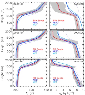
Since marine stratocumulus clouds are sensitive to boundary layer conditions, we first evaluate simulated vertical profiles of virtual potential temperature (θv) and water vapor mixing ratio (qv)with those observed by RB radiosondes and BAe-146 dropsondes (Fig. 1 and Table 3). The observed MBL is
Fig. 1. Vertical profiles of virtual potential temperature (θv) and water vapor mixing ratio (qv) measured by radiosondes released from the RB ship (red) and those from AERO (blue) and MET (light blue) simulations. The shaded area represents±1σ of the obser-vations. The dash blue lines also indicate the±1σ of the AERO simulations. Numbers of observational profiles used for the averag-ing are 31, 54, and 23 for panels in top, middle, and bottom rows, respectively.
more well-mixed over the coastal region than over the remote marine region. As evident in observed profiles over the re-mote region, there is more frequent decoupling (Zuidema et al., 2009) within the MBL over the remote region that sep-arates the well-mixed cloud layer from the subcloud layer. The coastal region has a stronger temperature inversion with a 10–12 K increase inθvwithin inversion layers (also see Ta-ble 3). The mean observed humidity and temperature in the MBL over the coastal and the remote regions, however, are not statistically different (at 98 % confidence level) between the two regions.
Table 3.Observed and simulated MBL temperature and humidity, 10-m wind speed, SST, and boundary layer height.
Variable Platform/ Coastal regiona Remote regiona Both regions (Units) Simulations Mean/Std Mean/Std Mean/Std
Temperature, humidity, and MBLHd,e
θv(K)b
RB 290.9/0.9 291.2/0.6 291.0/0.8 AERO 290.3/1.2 290.7/0.6 290.4/1.1 MET 290.0/1.1 290.9/0.6 290.6/1.0
BAe-146 290.6/0.8 – –
AERO 291.3/1.2 – –
MET 291.4/1.0 – –
qv
RB 7.9/0.7 8.1/0.7 7.9/0.7
(g kg−1)b
AERO 8.3/0.7 8.4/0.7 8.4/0.7
MET 8.2/0.8 8.0/0.6 8.2/0.7
BAe-146 8.0/0.6 – –
AERO 9.1/0.7 – –
MET 9.1/0.9 – –
dθv/dhc
RB 39.7 20.0 –
(K km−1)
AERO 29.6 17.9 –
MET 23.0 23.9 –
BAe-146 30.4 – –
AERO 24.7 – –
MET 21.8 – –
dqv/dhc
RB −16.8 −12.9 –
(g kg−1km−1)
AERO −11.6 −12.1 –
MET −8.2 −12.5 –
BAe-146 −11.2 – –
AERO −6.0 – –
MET −5.1 – –
MBLH (m)
RB 1263/113 1431/163 1313/151 AERO 1136/153 1398/186 1213/202 MET 1197/189 1686/139 1343/285
BAe-146 1122/130 – –
AERO 1051/168 – –
MET 1133/184 – –
Winds, SST
U10(m s−1)f
RB 4.8/1.3 8.2/1.3 6.2/2.1
AERO 4.9/1.6 8.8/1.1 6.4/2.4
MET 4.8/1.4 8.8/1.2 6.4/2.3
SST (K)
RB 291.2/0.9 291.7/0.6 291.4/0.8 AERO 290.9/0.5 291.7/0.5 291.3/0.6 MET 290.9/0.5 291.7/0.5 291.3/0.6
Accumulation mode aerosol (0.156–2.69 µm) concentration
Na(cm−3) C-130 243/147 105/95 184/144
AERO 160/68 81/36 126/68
Droplet number concentration
Nd(cm−3)
C-130 203/84 85/55 154/93
AERO 160/94 75/56 124/90
DMS transfer velocity (Kw), MBL DMS and SO2air concentrations
Kw(cm h−1) RBAERO 3.80/1.966.29/3.53 15.85/3.769.04/2.95 5.69/3.449.73/5.85
DMS Air (pptv) RB 43.2/27.5 78.2/21.6 56.9/30.6 AERO 138.4/49.6 216.5/41.0 169.1/60.1
SO2air (pptv)
C-130 54.0/74.5 27.8/18.7 40.8/55.7 AERO 38.8/71.6 11.8/17.3 25.2/53.6
aCoastal and remote regions are defined as east and west of 78◦W within the model domain, respectively.bFor the lowest 1 km within MBL.cFor the inversion layer.dIncluding
23 and 54 (RB) radiosonde profiles over the remote and coastal regions, respectively.eIncluding 31 (BAe-146) dropsonde profiles over the coastal region.fthe value for the RB is
from both simulations, on average, are biased high within MBL (biases of 0.4–1.1 g kg−1) and in lower free tropo-sphere (above MBL and <2 km, biases of 1.6–2.2 g kg−1) with more significant biases seen in the comparisons with the dropsondes. The larger biases in AERO and MET com-pared to the dropsondes are associated with the larger bi-ases in model predictions during 2–10 November, when the observed temperature inversion is weaker and the vertical variability in humidity is large (with the possible presence of multi-cloud layers). Toniazzo et al. (2011) also noted early November to be a period with reduced synoptic-scale vari-ability, lower inversion heights and increased cloud cover. The RB had measurements on 2–3 November before a 6-day break in sampling and the mean profiles were less affected by profiles measured during this synoptic episode. Over the remote region, the simulated mean temperature and humid-ity are in excellent agreement with AERO simulations with the simulated mean values being not statistically different (at 98 % confidence level) from observations at most vertical layers from the surface to 2 km. Over this region, the biases of the simulated mean profile in MET are mostly within the inversion layer.
As shown in Table 3 and Fig. 1, the AERO simulation bet-ter predicts the temperature and humidity gradients within the inversion layer than the MET over both regions, except for the humidity gradient over the remote region.
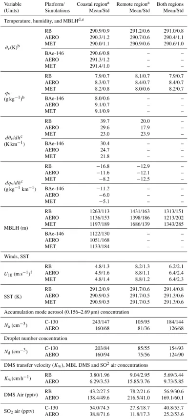
The zonal and diurnal variations of predicted MBL depths are compared to those from the RB and BAe-146 observa-tions, as shown in Fig. 2 and Table 3. Since BAe-146 drop-sonde data were released within a narrow time window dur-ing the day (14:00–16:00 UTC), they have not been included in the diurnal variability plot (bottom panel of Fig. 2). In simulations using the YSU PBL scheme, clouds often form on top of the on-line diagnosed PBL heights. Therefore, the MBL depth is determined as the lowest height where the lo-cal temperature gradient is at least 3 times the gradient be-low it. When a reasonable MBL depth is not found using this approach, the MBL depths for both model simulations and observations are determined from humidity profiles in a similar manner. The clear longitude dependence of observed MBL depths (in the range of 900–1600 m), which deepen far-ther away from the coast, is also reflected in both AERO and MET simulations (Fig. 2). The MBL depth from the MET simulation has a positive bias of∼250 m (Table 3) over the remote region. Inclusion of interactive aerosols in the AERO simulation leads to a lower MBL than in MET, giving bet-ter agreement with observations over the remote region (Ta-ble 3). However, the mean MBL depth from AERO is ap-proximately ∼100 m too low over the coastal region com-pared to radiosondes and dropsondes. The lower simulated MBL depths when aerosols are included are linked to the re-duction of MBL top entrainment and mean subsidence rates which are discussed later in more detail. The WRF sim-ulations described by Rahn and Garreaud (2010) using the Mellor-Yamada-Janjic PBL scheme had lower MBL depths
Fig. 2.Longitudinal and diurnal variations of the MBL heights de-rived from the RB radiosonde and BAe-146 dropsonde measure-ments (red), and from the AERO (blue) and MET (light blue) simu-lations. Only radiosonde profiles are included in the bottom panel. The MBL heights are determined from temperature profiles in com-bination with humidity profiles. The numbers of observational data used are indicated below the data points.
than observations, which is consistent with our results near the coastal region but not over the remote region. This might be due to differences in model setup, including the use of a different PBL scheme. As with Rahn and Garreaud (2010), the low bias in the mean MBL depth near the coast in both AERO and MET simulations could be explained by an over-prediction of low-level onshore wind speeds which lead to high biases in low-level divergence over a several hundred meter vertical layer resulting in lowering of MBL heights.
No significant diurnal variations in MBL depth are ob-served or modeled (bottom panel of Fig. 2). The lack of distinct diurnal variations in MBL depth is consistent with Zuidema et al. (2009) and Rahn and Garreaud (2010) that describe weak dependence of MBL depth on air-sea tempera-ture differences. In addition, there is considerable day-to-day and spatial variability in MBL heights as reflected in stan-dard deviations (σ=151 m for the radiosonde observations; σ=202 m and 285 m for the AERO and MET, respectively).
3.2 Aerosol and cloud droplets
3.2.1 Aerosol and cloud droplet number concentrations
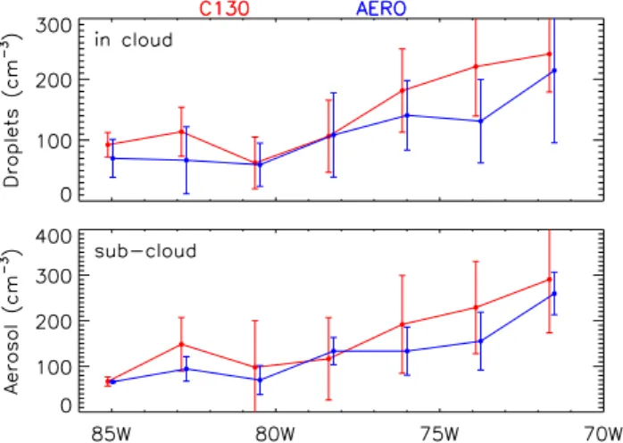
Fig. 3.Droplet number concentrations in the cloud layer and aerosol number concentrations in the sub-cloud layer observed on the C-130 aircraft (red) and predicted by the AERO simulation (blue). The aerosol size range is 0.156–2.69 µm in diameter for observations and 0.156–2.5 µm for the model. The error bar represents±1σ.
Observed aerosol and cloud droplet number concentrations both have strong longitudinal gradients over the coastal re-gion. As shown in the bottom panel of Fig. 3, the observed Nain the sub-cloud layer (on average 170 m above sea sur-face) is 290±117 cm−3 just west of the coast (71–72◦W),
decreasing to 117±93 cm−3at∼78◦W. The mean observed
concentration over the remote region is 105±95 cm−3 (Ta-ble 3). The modeled Na in the sub-cloud layer resembles the observed in longitudinal variation. However, simulated Naconcentrations (from model size bins 3–6) are lower than observations with mean biases of 34 % and 23 % over the coastal and remote regions, respectively. The predicted size distribution peaks at model size bin 2 (0.08–0.16 µm in di-ameter), and the number concentration in model size bin 2 is about 1.5 times the modeledNa concentration (includes model bins 3–6). Thus, errors in the size distribution could contribute to the number bias. Given the multitude of source and sink processes that affect aerosol number concentrations, the∼30 %Nabias is quite good.
Overall, simulated and observed cloud droplet number concentrations exhibit the same longitudinal gradient as that of the aerosol. This is expected, since hygroscopic aerosol particles acting as CCN can activate and form new cloud droplets. The observedNd has a mean value of 240 cm−3 near the coast and decreases to below 120 cm−3at∼78◦W,
and further decreases to a mean value of 85±55 cm−3over the remote region. The observed longitudinal variation inNd is in general agreement with the variation shown in Fig. 11 of Allen et al. (2011) in which CDP measurements on both the BAe-146 and C-130 were included. The domain aver-age near-surfaceNdof 154 cm−3measured by the C130 (Ta-ble 3) is in-between the meanNd values of 164 cm−3 and 142 cm−3based on aircraft and MODIS measurements dur-ing the VOCALS-REx obtained by Bretherton et al. (2010b),
in which their focus region was along 20◦S and multiple
air-craft measurements ofNdwere included. The modeled cloud droplet concentrations are lower by 21 % and 13 % over the coastal and the remote regions, respectively, which is related to the low biases in the predicted aerosol concentrations.
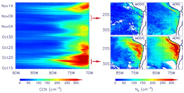
Aerosol, CCN and cloud droplet number concentrations over the SEP are strongly influenced by pollution outflow from the continent. In Fig. 10 of Bretherton et al. (2010b), daily MODIS-derived Nd were compared against aircraft measurements, and it showed the occurrence of a few strong outflow events along 20◦S over the SEP. The longitude-time plot of model (AERO) predicted CCN concentrations (at 0.1 % supersaturation) at 975 hPa are shown in Fig. 4 (left panel). The model succeeds in capturing the timing and strength of the observed outflow events shown in Fig. 10 of Bretherton et al. (2010b). During the VOCALS-REx, the strongest pollution outflow event along 20◦S peaked on 18
October, and the cleanest period was around 8 November. The four contour plots on the right panel of Fig. 4 illustrate the horizontal distribution of MODIS-derived (using Eq. (2) of George and Wood, 2010) and model-predictedNdduring the two time periods, respectively. Model simulatedNd com-pares reasonably well with observations. The model repro-duces the outflow pattern from coastline towards the ocean with a band of high Nd several-degrees wide in longitude along the coast. Considering the relatively large uncertain-ties in satellite-derivedNddue to averaging over only several instantaneous satellite snapshots and the timing differences between satellite overpasses and model outputs, the agree-ment in the outflow patterns is remarkably good. The model also capturesNdspatial patterns during the clean event. The accurate predictions of both events demonstrate the model’s ability to capture daily/synoptic scale variations of aerosol and clouds, and suggest that the model is suitable for stud-ies at such scales (e.g., pollution outflow studstud-ies), which is another advantage of using WRF-Chem with the prognostic treatment of aerosols and cloud-aerosol interactions.
3.2.2 Aerosol mass and composition
Fig. 4. Longitude-time plot of model (AERO) predicted CCN (at 0.1 % supersaturation) concentrations at 975 hPa along 20◦S (±2.5◦in latitude), and illustration of episodic horizontal distribution of MODIS-derived (Aqua) cloud droplet number concentration (Nd)and
AERO-predicted cloud topNdduring a strong outflow event (peaks on 18 October 2011, red solid line) and during a clean period (around 8 November 2011, red dash line). To obtain a more complete data coverage over the domain, MODISNdwas composed from available retrievals in 3 days (centered at the peak of the event), and correspondingly only model predictions at around satellite overpass time (18:00–20:00 UTC) during the 3-day period are included.
The predicted non-sea-salt submicron sulfate concentra-tions over the coastal region are roughly 37 % and 15 % lower than the observed values, which are 0.85 µg m−3 and 1.13 µg m−3 based on the AMS instruments onboard the C-130 and RB, respectively. The AMS and PILS on the G-1 measured sulfate concentrations of 1.10 µg m−3 and 1.29 µg m−3, respectively. Over the coastal region, the high mean sulfate concentration (1.81 µg m−3, Table 4) measured by the AMS on the BAe-146 is dominated by the high values (mean of 2.82 µg m−3)in a pollution plume study flight on 10 November 2008. Excluding this flight, the mean sulfate concentration (1.13 µg m−3)over the coastal region observed on the BAe-146 is in close agreement with those measured on the RB and C-130 (Table 4), which is underpredicted by 30 % in AERO. Observed submicron sulfate concentrations from different platforms are 0.27–0.39 µg m−3(Table 4) over the remote region. These observed values over both coastal and remote regions are in general agreement with those in Fig. 8 of Allen et al. (2011). Over the coastal region, the higher mean sulfate concentration from the RB in Table 4 compared to Fig. 8 of Allen et al. (2011) is mostly because we only used the RB observations within the VOCALS-REx period (15 October–15 November), which is a subset of the RB observations. For the supermicron sulfate, observations from the CIS on the RB show similar values (∼0.55 µg m−3) between remote and coastal regions. The simulated super-micron sulfate was in good agreement (∼20 % lower) with those observed on the RB over the coastal region, but was 80 % lower over the remote region. The larger bias over the
remote region suggests the underestimation of sulfate from DMS oxidation or too rapid sulfate removal, as addressed in more detail later in Sect. 4.
For ammonium mass concentrations, the simulated val-ues are significantly smaller than the corresponding measure-ments for both the submicron (0.07–0.09 µg m−3 vs. 0.11– 0.37 µg m−3) measured on different platforms and supermi-cron sizes (0.08 µg m−3 vs. 0.23 µg m−3) measured on the RB over the coastal region (Table 4). Over the remote re-gion, the detected ammonium concentrations (Table 4) are only slightly above instrument detection limits. The differ-ences between values observed on the RB and those of the C-130 over this region may reflect the difference in instru-ment detection limits. The corresponding predicted submi-cron ammonium is also small (<0.03 µg m−3) over the re-mote region.
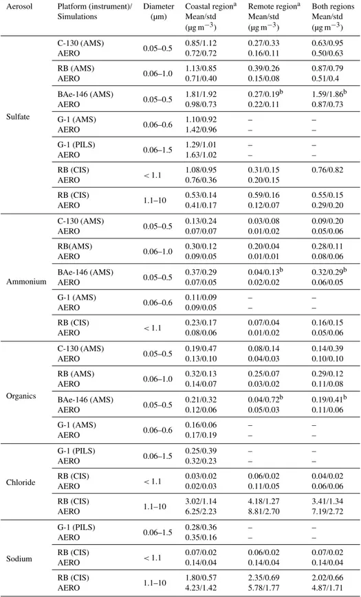
Table 4.Observed and simulated MBL submicron and supermicron aerosol composition.
Aerosol Platform (instrument)/ Diameter Coastal regiona Remote regiona Both regions Simulations (µm) Mean/std Mean/std Mean/std
(µg m−3) (µg m−3) (µg m−3)
Sulfate
C-130 (AMS)
0.05–0.5 0.85/1.12 0.27/0.33 0.63/0.95 AERO 0.72/0.72 0.16/0.11 0.50/0.63
RB (AMS)
0.06–1.0 1.13/0.85 0.39/0.26 0.87/0.79 AERO 0.71/0.40 0.15/0.08 0.51/0.4
BAe-146 (AMS)
0.05–0.5 1.81/1.92 0.27/0.19
b 1.59/1.86b
AERO 0.98/0.73 0.22/0.11 0.87/0.73
G-1 (AMS)
0.06–0.6 1.10/0.92 – –
AERO 1.42/0.96 – –
G-1 (PILS)
0.06–1.5 1.29/1.01 – –
AERO 1.63/1.02 – –
RB (CIS)
<1.1 1.08/0.95 0.31/0.15 0.76/0.82 AERO 0.76/0.36 0.20/0.15
RB (CIS)
1.1–10 0.53/0.14 0.59/0.16 0.55/0.15 AERO 0.41/0.17 0.12/0.07 0.29/0.20
Ammonium
C-130 (AMS)
0.05–0.5 0.13/0.24 0.03/0.08 0.09/0.20 AERO 0.07/0.07 0.01/0.02 0.05/0.06
RB(AMS)
0.06–1.0 0.30/0.12 0.20/0.04 0.28/0.11 AERO 0.09/0.05 0.01/0.01 0.08/0.06
BAe-146 (AMS)
0.05–0.5 0.37/0.29 0.04/0.13
b 0.32/0.29b
AERO 0.07/0.05 0.02/0.02 0.06/0.05
G-1 (AMS)
0.06–0.6 0.11/0.09 – –
AERO 0.09/0.05 – –
RB (CIS)
<1.1 0.23/0.17 0.07/0.04 0.16/0.15 AERO 0.08/0.06 0.01/0.02 0.05/0.06
Organics
C-130 (AMS)
0.05–0.5 0.19/0.47 0.08/0.14 0.14/0.39 AERO 0.13/0.10 0.04/0.03 0.10/0.10
RB (AMS)
0.06–1.0 0.32/0.13 0.25/0.07 0.29/0.12 AERO 0.14/0.07 0.03/0.02 0.11/0.08
BAe-146 (AMS)
0.05–0.5 0.21/0.32 0.04/0.72
b 0.19/0.41b AERO 0.12/0.06 0.05/0.03 0.11/0.06
G-1 (AMS)
0.06–0.6 0.16/0.06 – –
AERO 0.17/0.19 – –
Chloride
G-1 (PILS)
0.06–1.5 0.25/0.39 – –
AERO 0.32/0.23 – –
RB (CIS)
<1.1 0.03/0.02 0.06/0.02 0.04/0.02 AERO 0.02/0.03 0.11/0.05 0.06/0.06
RB (CIS)
1.1–10 3.02/1.14 4.18/1.27 3.41/1.34 AERO 6.25/2.23 8.81/2.70 7.19/2.72
Sodium
G-1 (PILS)
0.06–1.5 0.28/0.36 – –
AERO 0.35/0.16 – –
RB (CIS)
<1.1 0.07/0.02 0.06/0.02 0.07/0.02 AERO 0.14/0.04 0.14/0.04 0.14/0.04
RB (CIS)
1.1–10 1.80/0.57 2.35/0.69 2.02/0.66 AERO 4.23/1.42 5.78/1.77 4.87/1.71
aCoastal and remote regions are defined as east and west of 78◦W within the model domain, respectively.
Fig. 5.MBL submicron aerosol mass composition from VOCALS-REx measurements and from the AERO simulation. The measure-ments are provided by AMS instrumeasure-ments onboard the C-130, RB, and G-1 and those sampled by the CIS and a PILS onboard the RB and G-1, respectively. The pie charts and the total aerosol mass provided below them are based on the AERO simulation; only data along C-130 and RB tracks at the sampling time are included into the calculations. The dividing longitude for the coastal and remote regions is 78◦W, and the BAe-146 measurement data only covered the east edge of the remote region (78–81◦W with a mean longitude of 79◦W).
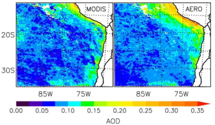
Fig. 6. AOD from MODIS (Aqua) measurements (left panel) and from the AERO simulation (right panel) during the VOCALS-REx period. Only model data at satellite scanning locations and times are included.
seawater. Chloride deficit was also observed on the RB dur-ing VOCALS-REx (Yang et al., 2011). We note that chloride deficit is well simulated by the AERO, but nitrate was under-predicted by∼50 % compared to the PILS.
The observed organic matter (OM) concentrations over the coastal region are 0.16–0.21 µg m−3 for smaller size (<0.6 µm) particles measured on the flight platforms and 0.32 µg m−3for the submicron particles measured on the RB.
The simulated values, on average, agree with that of G-1 within 6 %, while they are underpredicted in the model by 25–56 % compared to those on other platforms. Over the remote region, the C-130 and RB observed very different OM concentrations (0.08 µg m−3vs. 0.25 µg m−3), which are likely related to differences in sampling upper cutoff diame-ters and instrument detection limits. AERO does not include oceanic emissions of organic compounds, so the simulated ∼0.03–0.04 µg m−3OM over the remote region is solely due to continental sources. According to Hawkins et al. (2010), OM over the SEP has a dominant contribution from anthro-pogenic sources, and an additional, smaller contribution from primary marine sources based on measured functional groups and trace elements during VOCALS-REx. Lower OM con-centrations in MOSAIC could also result from the omission of secondary organic aerosol (SOA) formation processes. The contribution of SOA to OM is variable depending on fac-tors such as precursor concentrations, oxidant level, etc, and the organic mass associated with clean marine air (Hawkins et al., 2010).
The mean simulated chloride and sodium aerosol mass with diameter below 1.5 µm is in good agreement (∼25 % higher) with those sampled by the PILS (0.25 µg m−3 for chloride and 0.28 µg m−3for sodium) over the coastal region. The submicron chloride sampled on the RB has a domain-average of 0.04 µg m−3, which is overpredicted by ∼50 % in AERO (Table 4). The predicted supermicron chloride concentrations (6.25–8.81 µg m−3)are approximately twice the observed values (3.02–4.18 µg m−3)on the RB over the coastal and the remote regions (Table 4). The AERO pre-dicted sodium concentrations are also a factor of 2.0–2.4 higher than the RB observed values (Table 4). Note that the composition of freshly-emitted sea-salt particles reflects that of seawater, treating sea salt as NaCl in the model implies an overestimation of the sodium and chloride emissions by 25 % and 10 %, respectively. After accounting for this ef-fect, the supermicron sodium and chloride are overestimated by a factor of 1.9. The overestimation in the supermicron sizes could be related to errors in the predicted sea-salt size spectrum, which could also affect modeled dry deposition of larger particles.
As shown in Fig. 5, both observations and the simulation show 2–3 times higher total submicron mass concentration over the coastal region compared to the remote region. This highlights the importance of continental sources and the re-sulting outflow over maritime regions near the coast.
3.2.3 AOD
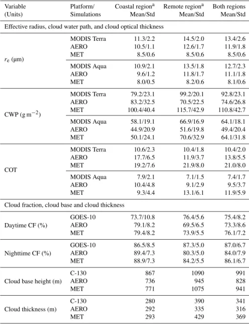
Table 5.Observed and simulated cloud properties.
Variable Platform/ Coastal regiona Remote regiona Both regions (Units) Simulations Mean/Std Mean/Std Mean/Std
Effective radius, cloud water path, and cloud optical thickness
re(µm)
MODIS Terra 11.3/2.2 14.5/2.0 13.4/2.6 AERO 10.5/1.1 12.6/1.7 11.9/1.8 MET 8.5/0.6 8.5/0.6 8.5/0.6
MODIS Aqua 10.9/2.1 13.5/1.8 12.7/2.3 AERO 9.6/1.2 11.8/1.7 11.1/1.8 MET 8.0/0.5 8.2/0.6 8.1/0.6
CWP (g m−2)
MODIS Terra 79.2/23.1 99.2/20.1 92.8/23.1 AERO 83.2/32.5 70.5/22.5 74.6/26.8 MET 100.4/40.4 115.7/42.9 110.8/42.7
MODIS Aqua 58.1/19.1 66.9/16.9 64.1/18.1 AERO 44.9/20.9 51.6/19.8 49.4/20.4 MET 50.1/24.1 70.6/32.9 64.1/31.8
COT
MODIS Terra 10.6/2.3 10.4/1.8 10.4/2.0 AERO 17.7/6.5 11.9/3.7 13.8/5.5 MET 19.2/7.6 21.9/8.0 21.0/8.0
MODIS Aqua 7.9/2.1 7.1/1.5 7.4/1.7 AERO 10.4/4.8 9.1/2.9 9.5/3.7 MET 9.3/4.4 13.1/6.1 11.9/5.9
Cloud fraction, cloud base and cloud thickness
Daytime CF (%)
GOES-10 73.7/10.8 76.4/5.6 75.4/8.2 AERO 79.1/8.2 69.5/6.5 73.3/8.6 MET 79.4/8.2 73.9/5.5 76.1/7.2
Nighttime CF (%)
GOES-10 86.5/8.5 87.3/5.0 87.0/6.7 AERO 89.4/7.3 80.3/5.0 84.0/7.9 MET 88.9/7.3 84.2/5.5 86.1/6.7
Cloud base height (m)
C-130 867 1090 991
AERO 736 945 828
MET 771 1075 941
Cloud thickness (m)
C-130 280 390 341
AERO 292 335 316
MET 293 429 369
aCoastal and remote regions are defined as east and west of 78◦W within the model domain, respectively.
general spatial features observed by the satellite quite well. The domain-average AODs are 0.10±0.06 and 0.11±0.06 for MODIS and the AERO simulation, respectively. Both the model and observations show that high AOD values (i.e., >0.2) are located along the coast, especially in a broad band with peak AOD values of approximately 0.3–0.4 off the northern Peruvian coast. The strong AOD gradient near the coast suggests influences from continental pollution out-flow, which is also consistent with the longitudinal variation of aerosol loadings from in-situ instruments (Fig. 3). Along-shore winds associated with high-pressure systems combined with the Andes that form a physical barrier lead to aerosol transport from continental sources such as Santiago, Chile, to the northern coastal region (Huneeus et al., 2006).
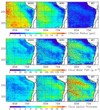
Fig. 7.Effective radius, cloud water path, and cloud optical thick-ness during the VOCALS-REx period from MODIS (Aqua) re-trievals and from the AERO and MET simulations.
Fig. 8. Mean low cloud fractions during day and night for the VOCALS-REx period retrieved from the GOES–10 (left), and those from the AERO (middle) and MET (right) model simulations.
3.3 Effective radius, cloud water path, and cloud optical thickness
Simulated cloud optical properties, which are cloud top ef-fective radius (re), cloud water path (CWP), and cloud optical thickness (COT), are compared against those from MODIS. As shown in Fig. 7 and Table 5, AERO results, in general, agree better with observations than do MET results for these three cloud properties.
MODIS re has a distinct longitudinal gradient north of 30◦S (Fig. 7) with values increasing from∼8 µm right off
the coast to>16 µm near 90◦W. This spatial distribution is
consistent with the AOD gradient shown in Fig. 6. A simi-lar longitudinalregradient is simulated in AERO, though the largeresouth of 30◦S is not well captured in the model. The domain-averagere(Table 5) values are∼13 µm for MODIS
observations on the Terra and Aqua, and are 11–12 µm for AERO. In comparison, MET substantially underestimated re(∼8–9 µm), due to the use of the default, constant cloud droplet number concentration of 250 cm−3, which is repsentative of the conditions near land (Fig. 3). Although re-ducing the constantNdof 250 cm−3to a more representative average droplet number concentration of 150 cm−3increases domain-averagereby 14 %, the uniform droplet number con-centration in MET still limits the spatial and temporal vari-ability ofre.
The domain averages of CWP are 93 and 64 g m−2based on Terra and Aqua satellite retrievals, respectively. The AERO domain-average CWP values are underestimated by ∼20 % compared to both satellites. The MET predicted do-main averages of CWP are in good agreement with Aqua ob-servations in the afternoon, but are overestimated by 23 % compared to morning observations on the Terra. The CWP spatial variations (Fig. 7) are better simulated in AERO than in MET, and the strong diurnal variation as reflected by the 45 % morning-to-afternoon decrease in domain-average CWP (based on the difference in Terra and Aqua observa-tions) is better simulated in AERO (51 % decrease) than in MET (73 % decrease). In AERO, the negative bias in CWP over the remote region might be related to the underpre-diction in droplet number. Low droplet number concentra-tions due to under-predicted aerosol concentraconcentra-tions result in shorter cloud lifetime. In MET, changing the constant Nd from 250 to 150 cm−3only reduces CWP by 3 % over the re-mote region, although the rain rate over this region increases by about 35 %; this is due to the very weak drizzle simulated in MET, which is discussed in more detail in Sect. 3.6.
Both AERO and MET overestimate the COT but with a substantially high bias (∼60–100 %) seen in MET (Fig. 7 and Table 5). The doubled COT in MET is related to its near constant smallre(10 µm) and the overestimated CWP that are used in calculating COT (i.e., COT ∼ cloud wa-ter content/re). The satellite-observed 40 %
3.4 Cloud fraction, cloud base, and cloud thickness
Figure 8 shows mean low cloud fractions retrieved from the GOES-10, and those in the AERO and MET during the VOCALS-REx. The presence of low clouds is diagnosed based on the criterion of cloud water mixing ratio exceed-ing a threshold of 0.01 g kg−1anywhere in a grid column be-low 700 hPa. The resulting cloud fraction for the column is then set to either 0 or 1. When averaging over the simulation period, the cloud fraction represents the frequency of cloud occurrence.
Satellite observations reveal more cloudiness during the night than during the day with a maximum located near 20◦S
and several degrees in longitude away from the coastline. AERO and MET broadly reproduce the day-night contrast as well as the northeast-southwest gradients in cloudiness as seen in satellite observations. The domain-average low cloud fraction from satellite is 75±8 % during the day and 87±7 % during the night (Table 5), which are well pre-dicted (<3 % biases) in both AERO and MET simulations with MET having slightly better agreement with observa-tions. While AERO mean cloud fractions are overestimated (3–4 %) over the coastal region, they are underestimated by 7 % over the remote region (i.e., near the south and west boundaries of the domain), as discussed in more detail in Sect. 4.
The near-coast minimum in low cloud fraction result-ing from enhanced orographic subsidence associated with synoptic-scale ridging (Toniazzo et al., 2011) is evident in GOES-10 data with minimum values around 15◦S and south of 20◦S along the coastline during the day. The nighttime near-coast minimum cloudiness appears at similar locations as in the daytime along the northern Chile coastline but with higher values. Both AERO and MET are able to capture the minimum cloud fractions at these locations but to a smaller spatial extent. An exception is along the coast south of 23◦S
where the simulated cloud fraction exceeds 80 % at night. Between the two minima, both the observed and simulated results show high cloud fractions along the coastline which are likely associated with the dynamical blocking of the sur-face wind by the southern Peruvian Andes, leading to con-vergence and a mean upward motion (Garreaud and Munoz, 2005).
Observations and simulations show that cloud thickness increases with distance from the coast. Both AERO and MET modeled cloud thickness are in excellent agreement with the observations (∼340 m), with ∼25 m low and high mean biases (Fig. 9 and Table 5), respectively. While the mean cloud base height from the C-130 over the remote re-gion (∼1100 m) is within the 1000–1200 m range (median) reported by Bretherton et al. (2010b) for their transition and remote regions, over the coastal region our observed mean cloud base height (∼900 m) is lower than their cloud base height (median, 1000 m), which is most likely due to their inclusion of only flight data along 20◦S. Cloud base heights
Fig. 9.Histogram of cloud thickness from the Wyoming cloud lidar (WCL) and radar (WCR) observations (red), and from the AERO (blue) and MET (light blue) simulations.
are better predicted in MET than in AERO. The underpredic-tion (∼160 m) of the mean cloud base height in AERO com-pared to observations on the C-130 is consistent with its low bias (mean bias of∼110 m) of MBL heights compared to ra-diosonde measurements on the RB. AERO does particularly well at simulating the frequency of clouds thicker than about 500 m, while MET overestimates these thicker clouds and underestimates clouds between 300 and 500 m thick (Fig. 9). In MET, when using a constantNdof 150 cm−3, cloud thick-ness is reduced by 20 m over the remote region, agreeing bet-ter with observations.
3.5 TOA and surface energy fluxes
Top-of-atmosphere (TOA) outgoing energy fluxes are modu-lated by water vapor, aerosol, and cloud properties, and sur-face energy fluxes are linked to SST, wind speed, air-sea tem-perature, humidity differences, and cloud forcing (de Szoeke et al., 2010). The simulated TOA outgoing SW fluxes are compared against those measured by the CERES onboard the Terra satellite (Fig. 10).
Table 6.Observed and simulated top-of-atmosphere (TOA) outgoing shortwave radiation and surface fluxes.
Variable Platform/ Coastal regiona Remote regiona Both regions
(Units) Simulations Mean/Std Mean/Std Mean/Std
TOA outgoing fluxes
TOA SW MODIS Terra 360.8/69.6 341.2/52.5 347.5/59.2
(W m−2) AERO 410.4/90.8 318.6/61.9 348.1/84.2
MET 395.8/90.9 376.9/70.8 383.0/78.3
Surface fluxes
Sensible heat RB 3.0/3.2 6.1/6.5 4.1/4.9
(W m−2) AERO 9.6/4.5 15.1/6.7 11.6/6.0
MET 7.4/3.5 10.3/5.6 8.5/4.6
Latent heat RB 76.5/23.9 115.5/30.5 90.7/32.4
(W m−2) AERO 76.6/25.2 140.7/34.7 100.0/42.4
MET 76.7/23.4 149.1/39.7 103.1/46.2
SW↓b RB 261.5/362.4 227.3/311.8 239.8/331.5
(W m−2) AERO 257.0/356.8 209.5/295.1 226.8/319.7 MET 222.3/336.0 238.2/323.9 232.4/328.4
LW↓b RB 373.7/21.4 364.9/25.6 370.2/23.5
(W m−2) AERO 376.0/17.9 362.5/29.1 371.1/23.6
MET 375.2/18.2 367.3/27.0 372.3/22.2
aCoastal and remote regions are defined as east and west of 78◦W within the model domain, respectively. bDownward fluxes.
Fig. 10. Top-the-atmosphere (TOA) outgoing shortwave (SW) ra-diation fluxes measured by the CERES (Terra) and those simulated in the AERO and MET simulations.
observed maximum. But the observed SW minimum along the coast near 15◦S is not well captured. For this particular region, although AERO simulated COT is smaller than obser-vations (Fig. 7), the impact of this negative bias on outgoing SW fluxes is compensated by overestimations of both AOD (Fig. 6) and cloud fraction (Fig. 8). In AERO, the biases in cloud fraction correlate well with the biases in TOA SW. For example, the low biases near the west boundary corre-spond to the underestimation of cloudiness in this region. In the MET simulation, TOA SW fluxes are overestimated by ∼10 % over both coastal and remote regions. The substan-tial overprediction of cloud optical thickness in MET (Fig. 8) also contributes to this high bias.
The TOA model-satellite comparison presents a regional view. Alternatively, a sonic anemometer onboard the RB monitored surface fluxes at a high time frequency (10 min) along the ship track allowing us to examine the associated longitudinal and diurnal variations (Fig. 11). The observed surface fluxes include sensible heat, latent heat, downward shortwave, and downward longwave fluxes (Table 6). Ob-served sensible heat fluxes are small (domain average of 4 W m−2) with a weak longitudinal gradient. The mean sen-sible heat flux is a small negative value at around 80◦W, and de Szoeke (2010) also noted the small sensible heat flux at 80◦W associated with the relatively small mean sea-air
tem-perature difference at based on a few years of cruise obser-vations along 20◦S. The sensible heat fluxes simulated by
AERO and MET are biased high with means of 12 W m−2 and 9 W m−2, respectively, and have a more distinct increas-ing trend towards the west. Associated with solar heatincreas-ing of the atmosphere, both observed and simulated sensible heat fluxes have a decreasing tendency from late morning to the afternoon (10:00–17:00 LT), although this decreasing ten-dency continues to late evening (22:00 LT) in the observa-tions but ends several hours earlier in the simulaobserva-tions.
Table 7.Observed and simulated in-cloud and near-surface rain rates.
Regions Platform/ Coastal regiona Remote regiona Both Regions (Units) Simulations Mean/Median Mean/Median Mean/Median
In-cloud C-130 0.668/0.112 6.891/0.396 3.704/0.161 (mm day−1) BAe-146 0.462/0.000 1.240/0.001
b 0.574/0.000b
AERO 0.037/0.013 0.163/0.052 0.099/0.019 MET 0.012/0.004 0.052/0.013 0.031/0.006
Near surfacec C-130 0.001/0.000 5.175/0.002 3.619/0.000 (mm day−1) BAe-146 0.001/0.000 0.279/0.000
b 0.014/0.000b
AERO 0.037/0.033 0.069/0.053 0.052/0.042 MET 0.023/0.018 0.059/0.044 0.040/0.027
aCoastal and remote regions are defined as east and west of 78◦W within the model domain, respectively.bThe BAe-146 measurement data only covered the east edge of the
remote region (78–81◦W with mean longitude of 79◦W).cBelow 300 m for BAe-146.
Fig. 11. Longitudinal and diurnal variations of surface fluxes in-cluding sensible heat, latent heat, downward shortwave, and down-ward longwave fluxes, from the sonic anemometer observations on the RB (red) and from the AERO (blue) and MET (light blue) simu-lations. The diurnal cycle of incoming shortwave fluxes is plotted as the difference between modeled and observed values. The vertical bars indicate±2σ, whereσ is the standard deviation of the mean value given byσ=pvar(xi)/n, where var(xi) is the variance of
data used for the averaging, and n is the number of the data points. Note that due to the large variability in some parameters,σ is not represented as the square root of the variance as in other figures.
al., 2011) increases from 4.8 m s−1over the coastal region to 8.2 m s−1over the remote region. The observed surface la-tent heat flux has a mean value of 91 W m−2. The mean latent heat flux from AERO (100 W m−2) shows a slight improve-ment from that (103 W m−2) of MET. The observed latent heat fluxes do not have a distinct diurnal variation; the simu-lated latent heat has biases which peak in the early morning.
The mean downward SW flux from the AERO agrees within 2 % with observations over the coastal region, and is ∼8 % lower over the remote region. The MET simulation underestimates SW fluxes by∼15 % over the coastal region, but overpredicts by 5 % over the remote region. The apparent better-predicted SW fluxes over the coastal region in AERO compared to MET indicate better-predicted daytime cloud cover along the path of the ship in AERO over this region. The diurnal variation of incoming SW fluxes in Fig. 11 is plotted as differences between modeled and observed values due to the large diurnal cycle. Both simulations tend to un-derpredict SW in the morning; AERO shows apparent better predictions than does MET in the afternoon. The analysis shown here is a direct comparison of observed and simulated data in corresponding times and locations and does not ac-count for the large instant biases in SW due to prediction bi-ases in instantaneous cloud field. Therefore, given this strict comparison, the results are quite good.
Predicted downward longwave fluxes and observations are in good agreement with mean differences of less than 1 W m−2. The observed downward longwave fluxes have a distinct diurnal variation with higher values (∼380 W m−2) at night and a minimum (∼350 W m−2) in the afternoon (15:00 LT). The AERO simulates a slightly better variation than does the MET during the day. The diurnal and longitudi-nal variations of the surface downwelling SW and LW fluxes are strongly associated with the corresponding variations in clouds.
3.6 Rain rate
median in-cloud and near-surface rain rate values are pre-sented in Table 7. In-cloud rain rates are averaged over the in-cloud flight legs with various depths in the cloud layer. The in-cloud and near-surface rain rates from the C-130 and BAe-146 agree within 30 % over the coastal region with the differences most likely associated with different particle size detection ranges of the instruments. This good agreement provides additional confidence in the derived rain rates from both 2D-C probes in this study. The rain rates over the re-mote region from the BAe-146 are much smaller than those measured by the C-130 and are not representative of the en-tire remote region since the BAe-146 2D-C measurements only covered a small longitudinal range over the east edge of the remote region (78–81◦W with mean longitude of 79◦W). Therefore, the rain rate discussion that follows is based en-tirely on C-130 observations.
Noticeable longitudinal gradients exist in observed in-cloud and near-surface rain rates (∼200 m above the ocean surface). Observed average in-cloud rain rates increase by about 10-fold (0.668 vs. 6.891 mm day−1)from the coastal to the remote region (Table 7). Overall, the longitudinal vari-ations in rain rates are captured in model simulvari-ations but pre-dicted rain rates are about an order of magnitude smaller than the observed values within the cloud layer (Fig. 12 and Ta-ble 7). Our calculated mean rain rates are higher than those of Bretherton et al. (2010b) derived from a different 2D-C probe and the maximum radar reflectivity. However, the me-dian values of our in-cloud and near-surface rain rates agree reasonably well with those of the radar derived rain rates in Bretherton et al. (2010b). We used the precipitation sizing data observed using the 25 µm resolution 2D-C probe which is more reliable than the other 10 µm resolution 2D-C probe on the C-130, of which the true resolution was later found un-stable (A. Schanot, personal communication, 2010). AERO produces higher rain rates than the MET, with the AERO me-dian rain rates being generally close to the 75th percentile of MET, resulting in closer agreement with observations for AERO.
In the near-surface layer, drizzle was barely observed over the coastal region. Over the remote region although the ob-served mean near-surface rain rate is∼75 % of the in-cloud value, the median rain rate in near-surface layer is drastically smaller than the in-cloud value (0.002 vs. 0.396 mm day−1). The observed strong near-surface/in-cloud contrast seen in median rain rates but not in the means could be explained by the skewed distribution of rain rates. Light rain occurs more frequently in the SEP stratocumulus, dominates the median value, and is associated with smaller mean raindrop size and relatively high evaporation rates below clouds. In contrast, the mean precipitation rate is dominated by relatively heav-ier rain, which is associated with larger mean raindrop size and hence relatively lower evaporation rates below clouds. In both simulations, the near-surface/in-cloud rain rate trasts are not well represented, although these observed con-trast might be larger than in reality due to a 62.5 µm lower
Fig. 12.Box and whisker plots of longitude-binned rain rates from in-cloud measurements (red) by a 2D-C probe onboard the C-130 aircraft and from corresponding in-cloud values in the AERO (blue) and MET (light blue) simulations. The bottom and top of the box are 25th and 75th percentiles. The median is shown inside the box. The 10th and 90th percentiles are shown by the dash outside the box. The open circles indicate outliers (lower than 10th or higher than 90th percentiles). The diamonds show the mean over all legs in each longitude bin. The numbers on the top indicate the number of data points used to produce the box and whisker plot.
raindrop cutoff diameter in measurements. Evaporation be-low cloud base might shrink raindrops to sizes smaller than 62.5 µm at the near-surface layer, which could not be de-tected by the 2D-C probe.
In addition, the model did not reproduce the large vari-ability in observed rain rates. The observed rain rates are as high as 100 mm day−1on some flight legs, as indicated by the outliers (red circles in Fig. 12), yet the modeled drizzle rates barely exceed 2 mm day−1. This is most likely a model reso-lution issue. The rain rates derived from flight data were av-eraged over about 9 km flight distance, which is comparable to our model horizontal grid size. However, the WRF model is known to actually resolve processes at scales about 7 times the horizontal grid spacing (Skamarock, 2004). Higher ver-tical and horizontal resolution simulations will be conducted in a follow-on study to explore this resolution issue.
4 Discussion
The predicted MBL depth has a 130 m reduction when aerosol-cloud interactions are included in the model simu-lation (i.e., in AERO). Processes at different scales influence MBL depths over the SEP. For example, large-scale subsi-dence tends to suppress the growth of MBL; the local change of MBL depth with time may be affected by the horizon-tal advection of temperature and moisture at the top of the MBL (Rahn and Garreauh, 2010); active turbulent mixing corresponds to a higher MBL, and entrainment deepens and dries the MBL (Wood and Bretherton, 2004; Zuidema et al., 2009). Lower MBL depths in AERO compared to MET in-dicate the active role of aerosol and aerosol-cloud interac-tions in modifying those MBL processes. The horizontally and temporally averaged subsidence rate in the layers above the MBL is consistently stronger in AERO than in MET; at 850 hPa, the average subsidence rate is 0.24 cm s−1 in AERO, which is about 0.015 cm s−1higher than in MET. The AERO-predicted MBL top entrainment rate (0.67 cm s−1)is about 24 % smaller compared to that of the MET simula-tion (0.88 cm s−1). The entrainment rate was estimated us-ing Eq. (4) of Yang et al. (2009) with 5-min model outputs of tracer concentrations. It is worth noting that the estimated entrainment rate is larger than the nighttime entrainment rate (0.4 cm s−1) estimated by Yang et al. (2009) using budget analysis of measured DMS during the VOCALS-REx. This is very likely due to vertical resolution near cloud top and in the inversion layer. LES model simulations show entrain-ment is very sensitive to the vertical resolution and generally use finer resolution (e.g., 5 m in Bretherton et al., 2010a) than in our simulations. However, there is no reason to expect that the bias (relative to the Yang et al. estimate) would dif-fer significantly between the AERO and MET simulations, so the 24 % difference in entrainment rates between the two simulations should be meaningful. The 130 m lower MBL depth in AERO, compared to MET, could thus be explained by the entrainment and somewhat stronger mean subsidence in AERO. The AERO, compared to MET, also produces im-proved moisture and temperature gradients in the capping in-version layer. The strengthening of the inin-version near the coast by including aerosol in the model is likely due to the atmospheric diabatic heating induced by the direct effect of the absorbing aerosols and the resulting semi-direct effect of enhancing cloud evaporation (Matsui et al., 2006; Dunion and Velden, 2004). Particularly, compared to the MET, the stronger inversion in the AERO leads to weaker entrainment and suppresses the vertical growth of the MBL.
Simulated MBL aerosol is evaluated against observations in number, mass composition, and optical properties. The ob-served strong gradient in accumulation mode (0.16–2.69 µm) aerosol number concentrations near the coast over the SEP region is also predicted reasonably well in the AERO simula-tion. The predicted accumulation-mode aerosol number has a low bias of about∼30 %, which is in rather good agree-ment for simulating aerosol number. The longitudinal varia-tion in droplet number, in general, corresponds to the spatial
variation in aerosols. Consistent with the underestimation of accumulation mode aerosol, the cloud droplet number con-centrations are also too low.
The well-simulated variability of Ndduring the polluted and clean episodes illustrate the capability of the model with prognostic aerosols in simulating variations of aerosol and clouds at daily/synoptic scales, and thus the model is suitable for studies at such scales.
Non-sea-salt sulfate is the dominant aerosol species in sub-micron mass concentrations over both coastal and remote re-gions within the SEP MBL. It is tempting to attribute the larger underprediction in sulfate mass over the remote re-gion compared to the coastal rere-gion (35–62 % vs. 11–37 %) to the underprediction of secondary sulfate produced from DMS oxidation. However, further investigation does not sup-port this explanation. The mean AERO-predicted DMS air mixing ratio is approximately a factor of 3 higher than the mean RB observations (Table 3) which can be partially ex-plained by the∼71 % overestimation of the DMS ocean-to-atmosphere transfer velocity (Kw). The high bias inKw oc-curs mainly at higher wind speeds (not shown), consistent with Blomquist et al. (2006). Another source of error is the setting of a constant oceanic DMS as in the VOCA model intercomparison specifications. However, given the transfer velocity overestimate, the prescribed seawater DMS would have to be unrealistically low to cause the sulfate bias. De-spite the high predicted DMS levels relative to observations, predicted MBL SO2mixing ratios are underestimated (11.8 vs. 27.8 pptv) over the remote region. Sensitivity tests show that most of the emitted DMS converts to SO2, which then converts to sulfate primarily via aqueous phase cloud chem-istry reactions. Speeding up the DMS gas-phase chemchem-istry lowers DMS air concentrations but has little impact on sul-fate (not shown). Therefore, the underestimation of sulsul-fate is unlikely due to modeled DMS emissions or oxidation. An alternate explanation is that wet removal of sulfate, particu-larly that just formed by cloud chemistry, is too rapid in the model, and this needs further investigation. The underesti-mation of sulfate near the coast is likely due to low biases in continental emissions and/or transport biases.