www.hydrol-earth-syst-sci.net/18/3855/2014/ doi:10.5194/hess-18-3855-2014
© Author(s) 2014. CC Attribution 3.0 License.
Hydroclimatic regimes: a distributed water-balance framework
for hydrologic assessment, classification, and management
P. K. Weiskel1, D. M. Wolock2, P. J. Zarriello1, R. M. Vogel1,3, S. B. Levin1, and R. M. Lent4 1US Geological Survey, Northborough, MA 01532, USA
2US Geological Survey, Lawrence, KS 66049, USA
3Department of Civil and Environmental Engineering, Tufts University, Medford, MA 02155, USA 4US Geological Survey, Augusta, ME 04330, USA
Correspondence to:P. K. Weiskel ([email protected])
Received: 1 February 2014 – Published in Hydrol. Earth Syst. Sci. Discuss.: 11 March 2014 Revised: 3 August 2014 – Accepted: 7 August 2014 – Published: 1 October 2014
Abstract.Runoff-based indicators of terrestrial water avail-ability are appropriate for humid regions, but have tended to limit our basic hydrologic understanding of drylands – the dry-subhumid, semiarid, and arid regions which presently cover nearly half of the global land surface. In response, we introduce an indicator framework that gives equal weight to humid and dryland regions, accounting fully for both vertical (precipitation+evapotranspiration) and horizontal (ground-water+surface-water) components of the hydrologic cycle in any given location – as well as fluxes into and out of land-scape storage. We apply the framework to a diverse hydro-climatic region (the conterminous USA) using a distributed water-balance model consisting of 53 400 networked land-scape hydrologic units. Our model simulations indicate that about 21 % of the conterminous USA either generated no runoff or consumed runoff from upgradient sources on a mean-annual basis during the 20th century. Vertical fluxes exceeded horizontal fluxes across 76 % of the conterminous area. Long-term-average total water availability (TWA) dur-ing the 20th century, defined here as the total influx to a landscape hydrologic unit from precipitation, groundwater, and surface water, varied spatially by about 400 000-fold, a range of variation∼100 times larger than that for mean-annual runoff across the same area. The framework includes but is not limited to classical, runoff-based approaches to water-resource assessment. It also incorporates and reinter-prets the green- and blue-water perspective now gaining in-ternational acceptance. Implications of the new framework for several areas of contemporary hydrology are explored,
and the data requirements of the approach are discussed in re-lation to the increasing availability of gridded global climate, land-surface, and hydrologic data sets.
1 Introduction
processes such as runoff generation and streamflow under specified baseline conditions (e.g., Vörösmarty et al., 2000; Döll et al., 2003; Milly et al., 2005; Oki and Kanae, 2006; Röst et al., 2008; Hoff et al., 2010; Hagemann et al., 2013). Subsequently, these models have been used to simulate hy-drologic responses to land-cover, water-use, and climate change, at a range of spatial and temporal scales.
It is important to note that the term “baseline” can no longer be equated, without qualification, with pristine, prede-velopment, or long-term-average conditions, largely because of two recent insights on the part of the hydrologic commu-nity. First, it is now broadly understood that the Industrial Revolution launched a new period of earth’s history – the Anthropocene epoch. During this epoch, human effects on the climate, the hydrosphere, and the land-surface portion of the earth system have become pervasive, though not neces-sarily equally distributed in space (Vogel, 2011; Vörösmarty et al., 2013; Savenije et al., 2014). The second insight is the renewed appreciation of the nonstationary component of hy-drologic processes (Milly et al., 2008; Matalas, 2012; Rosner et al., 2014). In light of these developments, we use the term “baseline” in this paper to denote an explicitly specified pe-riod of observational record, or of model simulation, that can serve as a basis for comparison with other periods character-ized by different climate, land-cover, or water-use conditions. In order to facilitate comparative analysis and communi-cation in the growing fields of comparative hydrology and global hydrology (Falkenmark and Chapman, 1989; Thomp-son et al., 2013), we suggest that a coherent new framework of quantitative water-availability indicators is needed. The purpose of this paper is to derive such a framework, using the landscape water-balance equation as the organizing prin-ciple. The framework is spatially and temporally distributed, compatible with existing water-balance models such as those cited above, and unbiased – in the sense of being equally ap-plicable to humid and dryland (Appendix A) regions. More-over, the framework is informed by both classical (runoff-based) and emerging perspectives on water availability, in-cluding the green- and blue-water paradigm now gaining ac-ceptance in the water management community (Falkenmark and Rockström, 2004, 2006, 2010; cf. Special Issue, J. Hy-drol., 384, 3–4, 2010). The green-blue paradigm contains critical insights, which we reinterpret for this paper. After deriving the new framework, we demonstrate it across a di-verse hydroclimatic region (the conterminous USA). Finally, we discuss the implications of the framework for hydrologic assessment, classification, and management.
2 Theoretical background 2.1 The landscape water balance
The water balance of a hydrologic unit (Fig. 1a) may be stated as follows:
P (1t )+Lin(1t )+Hin(1t )=ET(1t )+Lout(1t )
+Hout(1t )+dST/dt (1t ), (1) where P is precipitation, Lin,out is saturated landscape (ground-water+surface-water) inflows to, and outflows from a hydrologic unit,Hin,out=human inflows to and with-drawals from a hydrologic unit (Weiskel et al., 2007),ETis evapotranspiration, and dST/dt=[(P+Lin)−(ET+Lout)] is the rate of change (positive, negative, or zero) of total wa-ter storage in the soil moisture, groundwawa-ter, surface wawa-ter, ice, snow, and human water infrastructure of the hydrologic unit – with all terms averaged over a time period (or step) of interest,1t, in units of L3T−1 per unit area of the hy-drologic unit, or L T−1(see Table 2). Human flows (H
inand
Hout) and the artificial component of total storage are initially set equal to zero for development of the baseline framework of the present paper.
2.2 Green and blue water
Water availability may be viewed from either an open-system, hydrologic-unit spatial perspective (Fig. 1a) or from a semiclosed, catchment perspective (Fig. 1b, and Ap-pendix A). Working within the catchment spatial context of Fig. 1b, Falkenmark and Rockström (2004, 2006, 2010) re-fer to the outflow termsETandLoutas “green” and “blue” water flows, respectively, and explore the consequences of this distinction for land and water management. Precipita-tion, in their framework, is viewed as an undifferentiated in-flow term, and is therefore symbolized by white arrows in Fig. 1b.
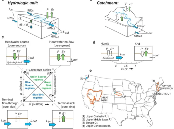
Figure 1. (a)Hydrologic unit, and(b)catchment, showing land–atmosphere (or green) fluxes (precipitation, evapotranspiration;P,ET)
and landscape (or blue) fluxes (groundwater+surface-water flows;Lin,Lout) at boundaries. Double arrows show change in green
(unsat-urated) and blue (sat(unsat-urated) storage; their sum equals change in total water storage (dST/dt) during a time step of interest. CatchmentP
influxes, defined by Falkenmark and Rockström (2004) as undifferentiated (neither green nor blue), indicated by white arrows. Internal soil
moisture/ groundwater/surface-water exchanges not shown.(c)Hydroclimatic regime for a hydrologic unit is defined by the 2-D, (et,p)
plotting position on central regime space; see Table 2 for et andpdefinitions. End-member regimes shown by sketches at corners of regime
space. Example regimes: sites 1, 2, 3, and 4; see Table 1.(d)Catchment hydroclimatic regime, defined by the 1-D position onET/P axis.
(e)Location map for sites 1, 2, 3, and 4 (Table 1), and major basins (Sect. 4; Fig. 2).
both types of inflow to a hydrologic unit (landscape inflows and precipitation) are available for partition into blue and green outflows.
2.3 Hydroclimatic regimes, total water availability, and regime indicators
We define the hydroclimatic regime of a hydrologic unit as the particular combination of green- and blue-water-balance components that characterizes the baseline functioning of a particular hydrologic unit (of any size) averaged over a spe-cific time step of interest (of any length). For the purposes of our initial theoretical analysis, human flows and artifi-cial storage are excluded from consideration, as noted above, and green and blue storage changes are lumped into a to-tal storage change term. Consistent with Milly et al. (2008), we also define hydroclimatic regimes in temporally explicit terms (i.e., for particular time periods or steps).
To facilitate the understanding of hydroclimatic regimes and the relative magnitudes of all water-balance
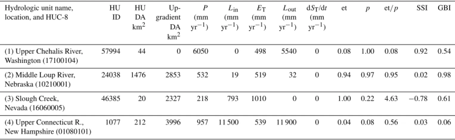
Table 1.Water-balance components and hydroclimatic regime indicators; sites 1, 2, 3, and 4 (Fig. 1e). The regime of each site approaches one of four end members shown in Fig. 1c. See Table 2 for indicator definitions. Mean-annual (1896–2006) water-balance components obtained from the distributed water-balance model of the conterminous USA (see Sect. 3). HUC-8 (eight-digit hydrologic-unit code; see Supplement); HU ID, hydrologic-unit identifier, water-balance model; DA, drainage area.P, precipitation;ET, evapotranspiration;Lin, landscape (surface
water+groundwater) inflow;Lout, landscape outflow; dST/dt, change in total landscape storage; all fluxes are per unit area of the local HU,
in units of millimeters per year; rounded to 3 significant figures. The terms et andp(normalized evapotranspiration and precipitation), et/p, (hydrologic-unitETratio), SSI (source-sink index), and GBI (green-blue index) are dimensionless; see Table 2.
Hydrologic unit name, HU HU Up- P Lin ET Lout dST/dt et p et/p SSI GBI
location, and HUC-8 ID DA gradient (mm (mm (mm (mm (mm km2 DA yr−1) yr−1) yr−1) yr−1) yr−1)
km2
(1) Upper Chehalis River, 57994 44 0 6050 0 498 5540 0 0.08 1.00 0.08 0.92 0.54 Washington (17100104)
(2) Middle Loup River, 24038 1476 2853 532 19 519 32 0 0.94 0.97 0.95 0.02 0.98 Nebraska (10210001)
(3) Slough Creek, 46385 20 2327 218 793 1010 0 0 1.00 0.22 4.63 −0.78 0.61 Nevada (16060005)
(4) Upper Connecticut R., 1077 212 3996 957 11 500 539 11 900 0 0.04 0.08 0.56 0.03 0.06 New Hampshire (01080101)
p+lin=et+lout+dsT/dt=1, when (dsT/dt >0); (2a)
p+lin+−dsT/dt=et+lout=1,when (dsT/dt <0) . (2b) Each term in Eqs. (2a) and (2b) represents a fraction of the total water balance, and the fractions on each side of the equations sum to 1. During periods of storage accretion (dsT/dt >0; Eq. 2a), the total storage change term may be treated as an outflow to storage. During periods of storage depletion (dsT/dt <0; Eq. 2b), the storage change term may be treated as an inflow from storage.
Hydroclimatic regimes may be represented graphically on plots of et versus p (Fig. 1c, central square). This square regime space comprises the full diversity of potential hy-droclimatic regimes found at earth’s land surface; the cor-ners of the plot correspond to end-member regimes where
p and et take on their limiting values. For example, at the headwater source end member (Fig. 1c),p=1, et=0,lin=0 andlout=1. At the pure-green, headwater no-flow end mem-ber, p=1, et=1, lin=0 and lout=0. At the terminal sink end member,p=0, et=1,lin=1 andlout=0. Finally, at the pure-blue, terminal flow-through end member,p=0, et=0,
lin=1 andlout=1. Example regimes 1–4 (Fig. 1c; with lo-cations shown on Fig. 1e) approach the respective end mem-bers. See Table 1 for the water budgets and hydroclimatic indicators associated with example regimes 1–4.
We use combinations of p and et to define a new set of hydroclimatic indicators (Table 2): the green-blue index (GBI=[p+et]/2), the hydrologic-unit-evapotranspiration ratio (et/p), and the source/sink index (SSI=p−et). The GBI indicates the relative magnitudes of green (P +ET) ver-sus blue (Lin+Lout) water fluxes experienced by a logic unit during a period of interest (see Table 2). A hydro-logic unit dominated by precipitation inflows and
evapotran-spiration outflows (headwater no-flow end member; Fig. 1c) has a GBI near 1, while a hydrologic unit dominated by landscape flows (terminal flow-through end member) has a GBI near 0. The remaining two indicators, SSI and et/p, dif-ferentiate runoff-generating source regimes (P > ET) from runoff-consuming sink regimes (ET> P), where sources of water forETinclude local precipitation, landscape inflows, and (on a transient basis) storage depletion. A hydrologic unit near the headwater-source end member (Fig. 1c) has an SSI near+1 and an et/pnear 0; a hydrologic unit near the termi-nal sink end member has an SSI near−1 and an et/p≫1, ap-proaching the local value of the aridity index (the long-term-average ratio of potential evapotranspiration [PET] toP).
Table 2.Indicators of terrestrial water availability.P, precipitation;ET, evapotranspiration; PET, potential evapotranspiration. Landscape
inflows and outflows (Lin,Lout) include both surface and groundwater flows (Fig. 1a). All length per time units (L T−1) are equivalent to
L−3L−2T−1, where L2refers to the area of the local HU that is receiving or donating water. LR is the mean local runoff during a specified long-term period; other indicators may be defined for a specified period, or time step, of any length.
Indicator Simple Expanded Measurement Permissible Reference
definition definition units range
Local runoff, LR P−ET same L T−1 ≥0 Bras (1989)
Landscape inflow,Lin Lin same L T−1 ≥0 this paper
Landscape outflow, Lout same L T−1 ≥0 this paper
Lout
Total storage dST/dt (P+Lin)−(ET+Lout) L T−1 positive, Bras (1989)
change, dST/dt negative, or zero
Aridity index, AI PET/P same dimensionless ≥0 Budyko (1974)
Catchment ET/P same dimensionless 0≤ETR≤1 Budyko (1974)
ETratio,ETR
Runoff ratio, RR 1−(ET/P ) same dimensionless 0≤RR≤1 Budyko (1974)
Total water – max{(P+Lin), L T−1 ≥0 this paper
availability, TWA ET+Lout+−dST/dt
Normalized p P /TWA dimensionless 0≤p≤1 this paper
precipitation,p
Normalized et ET/TWA dimensionless 0≤et≤1 this paper
evapotranspiration, et
Normalized total dsT/dt (dST/dt )/TWA dimensionless −1≤dsT/dt≤1 this paper
storage change
Source-sink index, p−et (P−ET)/TWA dimensionless −1≤SSI≤1 this paper
SSI
Green-blue index, (p+et)/2 (P+ET)/(P+ET+Lin dimensionless 0≤GBI≤1 this paper
GBI +Lout)
Hydrologic unit et/p ET,HU/P dimensionless ≥0 this paper
ETratio, et/p
3 Methods
3.1 Continental water-balance model and data sources An existing, distributed water-balance model of the conter-minous USA (McCabe and Markstrom, 2007) was modified to simulate baseline, mean-annual hydroclimatic regimes for the 1896–2006 period. The modified model allows for the consumption of groundwater and surface water in river corri-dors and terminal sink basins; it was developed by coupling a simple water-balance model to a river network. The mod-ified model was applied to the 53 400 networked hydrologic units defined by the individual segments of the river file 1 (RF1) river network (Nolan et al., 2002). Flow generated in the hydrologic units is routed downstream through the river network. Using the terms introduced in this paper, the Lin volume for a hydrologic unit equals the sum ofLoutvolumes
from the immediately upgradient hydrologic units. Depend-ing on climatic conditions, runoff consumption in a stream corridor or terminal-sink hydrologic unit (i.e., evapotranspi-ration of landscape inflows [Lin]) is allowed to occur to sat-isfy the evapotranspiration demand of a hydrologic unit. Note thatLinis a lumped term, comprising both groundwater and surface-water inflows to a hydrologic unit; see Fig. 1a, and Supplement.
major components of the hydrologic unit water budget in-cluding precipitation, PET, actual ET, snow accumulation, snowmelt, soil moisture storage, and runoff delivered to the stream network.
As streamflow is routed through the river network, some portion of the flow can be “lost” in a downstream hydrologic unit through evapotranspiration. The quantity of lost stream-flow is assumed to be a function, in part, of excess PETin the hydrologic unit, which is defined as theETthat is in excess of actualETcomputed by the water-balance model. The model assumes that excess PETwithin a river corridor places a de-mand on water entering the hydrologic unit from upstream flow and that the river corridor is 30 % of the total hydro-logic unit area. Furthermore, it is assumed that the amount of upstream flow that can be diverted to satisfy excess PET is limited to 50 % of the total upstream flow. The percentages used in the calculations were determined by subjective, trial-and-error calibration of the model to measured streamflow in arid-region river corridors that are known to lose water due to ground- and surface-water evapotranspiration in the down-stream direction. Runoff consumption in a hydrologic unit occurs when locally generated streamflow, computed from the water-balance model, is less than the computed stream-flow loss. For hydrologic units that are specified as termi-nal sinks in the RF-1 network, the total evapotranspiration from the hydrologic unit is set equal to total water available to the unit on a long-term-mean basis (P+Lin). In certain arid and semiarid hydrologic units of the conterminous USA, where no RF-1 stream reaches have been defined, we assume that long-term-mean precipitation (obtained from the PRISM data set) equals totalETfrom each unit, thatLin=Lout=0, and thatp=et=1. See Eqs. (1), (2), and associated text for definitions of terms.
The performance of the linked water-balance and river-network model was evaluated by comparing estimated streamflow to measured streamflow for river corridors with a complete data record for water-year 2004 (October 2003– September 2004). The correlation between estimated and measured mean-annual flow for all conterminous USA streamgages was 0.99. Correlation-coefficient values for selected river corridors with runoff-consuming hydrologic units were 0.75 (Colorado River), 0.98 (Missouri River), 0.99 (Yellowstone River), and 0.70 (Humboldt River). The lower correlation coefficients for some of the river corridors likely reflect the simplifying assumptions concerning runoff con-sumption used in this study (described above), the use of a lumped, landscape-flow approach (cf. Supplement), and the potential effects of human water use (Weiskel et al., 2007), which were not explicitly considered in this analysis.
3.2 Transient watershed model
A published watershed model of the Ipswich River basin, Massachusetts, USA (Zarriello and Ries, 2000), developed using the Hydrological Simulation Program-FORTRAN
(HSPF) code, was used to illustrate temporal variation in hy-droclimatic regimes. The published model was calibrated to observed daily streamflows at two long-term US Geologi-cal Survey streamgages in the basin (gages 01101500 and 01102000). For the purpose of our analysis, hourly model output values for the 1961–1995 period were aggregated to produce 420 consecutive monthly values of all water-balance components (Eq. 1) for a selected model hydrologic unit in the upper basin (Reach 6, Lubbers Brook). The resulting nor-malized regime indicators were then calculated and plotted at the monthly, median-monthly, and mean-annual timescales for the period of interest.
4 Results
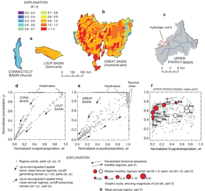
4.1 Spatial regime variation, conterminous USA In order to illustrate continental-scale spatial variation of long-term, mean-annual hydroclimatic regimes (both within and between individual river basins), we chose basins from humid, semiarid, and humid-to-arid regions of the contermi-nous USA for analysis. Maps of et/p, and plots of et vs.pare used to demonstrate spatial variation in mean conditions for the 20th century (Fig. 2a, b, d, e; see Fig. 1e for locations).
The plotted regimes (Fig. 2d) of the humid Connecticut River basin, New England (Fig. 2a), showed a roughly lin-ear pattern across the regime space, from headwaters (p=1) to mouth (p=0.0014). Runoff-generating regimes were in-dicated for the entire region; et/pranged from 0.28 to 0.64, as a function of elevation and latitude. Green flows exceeded blue flows (GBI>0.5) in 55 % of the 349 hydrologic units. Such moderate-source regimes (et/pnear 0.5) are common in humid, temperate regions where locally generated runoff is an important component of the landscape water balance.
The 150 hydrologic units of the semiarid Loup River basin, a subbasin of the Platte Basin in central Nebraska (Fig. 2a, d), had a median et/p ratio almost twice as large as the Connecticut Basin ratio (0.94 vs. 0.51). The ratios also varied over a narrower range (0.85–1.05). Consistent with the semiarid climate, 73 % of the hydrologic units in the Loup Basin were dominated by green regimes and 6.7 % were simulated as runoff-consuming on a long-term-average basis (ET> P, withLinmeeting a portion of the evapotran-spiration demand). The Loup River basin illustrates the low-runoff, P-and-ET-dominated hydroclimatic regimes com-mon to the semiarid steppes, savannas, and arid high deserts that comprise most of the world’s dryland ecosystems on all continents, from the subtropics to the midlatitudes (Reynolds et al., 2007).
Figure 2.Spatial variation of hydroclimatic regimes (1896–2006), shown by maps(a, b)of hydrologic-unit-evapotranspiration ratio (et/p)
and hydroclimatic-regime scatter plots(d, e)of selected USA basins: Connecticut River basin, New England (n=349); Loup River basin,
Nebraska (n=150); and Great Basin, intermountain USA (n=908). Temporal variation of monthly (n=420) median-monthly (n=12),
and mean-annual (n=1) hydroclimatic regimes (1961–1995) for hydrologic unit 6, Ipswich River basin, New England(c, f).
units near the eastern and western boundaries of the basin were runoff-generating, yet 29 % of the basin’s 908 hydro-logic units, and 34 % of its total area was runoff-consuming. The Great Basin is endorheic, or closed, under current cli-mate; all landscape flow paths ultimately terminate in low-land sinks where ET is the only outflow term in the wa-ter balance (et=1, right-vertical axis, Fig. 2e). Temporally averaged et/p varied 17-fold across the basin during the 20th century, from 0.28 in the High Sierras (western bound-ary) to 4.6 in Slough Creek in the central part of the basin (site 3 in Figs. 1c, 2e, and Table 1). The Great Basin is the major North American example of a closed,
humid-mountain-to-arid-lowland domain with extreme spatial vari-ation in hydroclimatic regimes. Comparable large endorheic systems include the closed basins of western China, the Aral and Caspian seas in central Asia, Lake Chad in cen-tral Africa, Lake Titicaca in Peru/Bolivia , and Lake Eyre in Australia (Zang et al., 2012; Micklin, 2010; Lemoalle et al., 2012).
quantitatively important for the landscape water balance (Nagler et al., 2009; Karimi et al., 2013). Such runoff-consuming landscapes (long-term et/p >1), comprise a sub-set of the world’s drylands with distinct hydroclimatic, eco-logical, and geochemical characteristics (Tyler et al., 2006; Nagler et al., 2009).
4.2 Temporal regime variation, Upper Ipswich Basin, New England, USA
Regime plots may also be used to display temporal regime variation, including storage dynamics, for individual hydro-logic units over a range of timescales. Using a previously published watershed model, we analyzed regime variations in a selected hydrologic unit (Fig. 2c) in the Upper Ipswich River basin, New England (see Methods Sect. 3.2). Regimes are plotted for the 420 consecutive months of the simula-tion period (1961–1995), and are aggregated to the median-monthly and mean-annual timescales (Fig. 2f). Simulated monthly et/pvaried by about 7000-fold and GBI by 30-fold over the period. Most of this variation can be attributed to the strongly seasonal ET cycle of the northeastern USA, since monthly precipitation is relatively constant year-round in the region (Vogel et al., 1999).
On a median-monthly basis over the study period, this hy-drologic unit generated runoff from September to May, and consumed runoff from June to August. Blue fluxes (Lin,Lout) dominated the water balance from October to June, while green fluxes (P,ET) dominated from July to September. Ac-cretion of total storage occurred from September to Febru-ary, and depletion of storage from March to August. Large seasonal and interannual hydroclimatic variation is indicated (Fig. 2f) in a region where spatial variation in hydroclimate is modest on a mean-annual basis (Vogel et al., 1999). The size, shape, and orientation of the regime point-cloud and median-monthly polygon (Fig. 2f) illustrate the seasonal dynamics of the various water-balance components (P,ET,Lin,Lout, dST/dt) and capture the hydrologic functioning of this hy-drologic unit over the 35-year period of interest.
5 Discussion
5.1 Implications for water-resource assessment
Classical hydroclimatic indicators such as local runoff, the aridity index, and the catchment evapotranspiration ratio (Ta-ble 2) have been used for decades in water-resource assess-ments at all spatial scales (Budyko, 1974; Gebert et al., 1987; Vogel et al., 1999; Sankarasubramanian and Vogel, 2003; Milly et al., 2005). The regime indicators of this pa-per complement these classical indicators and address some of their limitations as indicators of water availability. Be-low, we demonstrate how our new indicators (total water availability, the green-blue index, and the
hydrologic-unit-evapotranspiration ratio) address the limitations of two clas-sical indicators – local runoff and the aridity index.
5.1.1 Local runoff, total water availability, and the green-blue index
Maps of local runoff, constructed by contouring long-term, temporally averaged runoff (P−ET) values assigned to the centroids of gaged catchments (e.g., Gebert et al., 1987) effectively capture one aspect of hydroclimatic variation in runoff-generating regions; local runoff varied ∼ 3300-fold across the conterminous USA on a long-term, mean-annual basis during the 20th century (Figs. 3a; S1a in the Supplement). However, equating water availability for hu-mans and ecosystems with local runoff can hinder the ba-sic understanding of water availability (cf. Falkenmark and Rockström, 2004). A runoff-focused approach minimizes the role of precipitation as a source of water to landscapes, especially in semiarid regions with moderate precipitation (∼250–500 mm yr−1), comparably high evapotranspiration, and very low (or zero) runoff (e.g., Table 1, site 2). In ad-dition, maps of local runoff (Fig. 3a) neglect the networked character of water availability, that is, the role of hydrologic position (see Appendix A) as well as local climate in govern-ing the total amount of water available as inflow to a land-scape hydrologic unit. These limitations are addressed by our newly introduced TWA indicator (Eq. 2, Figs. 3b, S1a), and dimensionless GBI (Figs. 3d, S1c). The TWA indicator in-corporates both vertical (green), and horizontal (blue) com-ponents of inflow to a hydrologic unit, in units of volumetric inflow to the hydrologic unit per unit area of the receiving hydrologic unit (L−3L−2T−1, or L T−1). Because both pre-cipitation and landscape inflows are incorporated into TWA, it is an exceptionally sensitive indicator, and can vary spa-tially over a large range. In the conterminous USA, for ex-ample, TWA varied spatially by nearly 5 orders of magnitude (∼450 000-fold) on a mean-annual basis during the 20th cen-tury (Figs. 3b, S1a). At the low end of the TWA spectrum are found arid upland hydrologic units with low precipitation and no significant blue-water inflow (TWA<102mm yr−1); at the high end, hydrologic units at the mouths of large rivers (TWA>106mm yr−1, essentially all from blue-water inflow).
Figure 3.Classic(a, c, e)and newly introduced(b, d, f)indicators of terrestrial water availability for 53 400 networked hydrologic units of
the conterminous USA, on a mean-annual basis for 1896–2006. See text and Table 2 for indicator definitions.(a)Local runoff (mm yr−1),
5.1.2 Aridity index and the hydrologic-unitETratio
(et/p)
The aridity index (AI), the long-term-average ratio of poten-tial evapotranspiration to precipitation at a location (PET/P) is commonly used to show spatial variation in potential energy available for evapotranspiration (Sankarasubrama-nian and Vogel, 2003), estimate actual evapotranspiration (Budyko, 1974), and map the global distribution of dry-lands (UNEP, 1997). The main limitation of the aridity index (Figs. 3e, S1d) is that it fails to distinguish two basic dry-land types: (a) updry-lands whereETdemand is met strictly by soil moisture derived from local precipitation; and (b) runoff-consuming lowlands where ET demand is met by a com-bination of local precipitation, as well as groundwater and surface water derived from upgradient hydrologic units. The hydrologic-unit-evapotranspiration ratio (et/p; Figs. 3f, S1e) complements AI by quantifying actual rather than potential
ETrates across the full range of PETvalues found in a region. Maps of et/p allow for a more realistic representation of runoff-consuming, arid lowlands (both endorheic sinks and runoff-consuming river corridors) than maps of the aridity index alone.
For example, our et/pmap (Fig. 3f) indicates an east–west pattern of weak-sink river corridors in the High Plains of the central USA. When compared to an aridity map of the re-gion (Fig. 3e), the et/pmap suggests that spatial variation in the High Plains actual evapotranspiration in the 20th cen-tury was likely governed as much by the local geography of its river corridors – and the availability of blue water from Rocky Mountain-source areas to the west – as it was by lon-gitudinal variations in PETand precipitation alone. It is im-portant to note that the areal extent and magnitude of runoff consumption in a river corridor (under either predevelop-ment or developed conditions) depends on the spatial scale of averaging. The relatively coarse scale used our continental analysis (∼138 km2hydrologic units) may overestimate the spatial extent, and underestimate the local magnitude, of ac-tual runoff consumption by evaporation and by transpiration through riparian vegetation in individual High Plains river corridors. Improved quantification ofETusing remote sens-ing techniques and other methods could help to address this limitation (Nagler et al., 2009; Karimi et al., 2013; Sanford and Selnick, 2013).
5.2 Implications for hydrologic classification
The development of a coherent hydrologic classification system is widely recognized as a critical need within hy-drology (McDonnell and Woods, 2004; McDonnell et al., 2007; Sawicz et al., 2011; Toth, 2013; cf. Special Issue on Catchment Classification; Hydrol. Earth Syst. Sci., vol. 15, 2011). However, there is presently no quantitative, gener-ally accepted classification system that both encompasses the world’s hydrologic diversity and allows for quantitative
spec-ification of hydrologic thresholds and similarities, in a man-ner comparable to the dimensionless Reynolds and Froude numbers used to classify hydraulic systems (Wagener et al., 2007, 2008). Most researchers have focused their classifica-tion efforts on catchments (watersheds, basins) and their hy-drologic function (cf. summary by Sawicz et al., 2011). Oth-ers have focused on the conceptualization and classification of hydrologic landscapes (Winter, 2001; Wolock et al., 2004), lakes (Martin et al., 2011), or wetlands (Brinson, 1993; Lent et al., 1997).
In this section, we propose a hydrologic classification that uses the water balance of a hydrologic unit, i.e., Eq. (1), as its organizing principle. This approach encompasses both catch-ments (Lin=0;p=1) and all types of noncatchment sys-tems (Lin>0;p <1), such as wetlands, lakes, stream corri-dors, upland landscape units, and aggregations of hydrologic units (i.e., hydrologic landscapes).
5.2.1 A new classification of hydroclimatic regimes We begin the classification by specifying the local climate (et/p) of a hydrologic unit during a period of interest. The et/pindicator is used to define four regime classes (Fig. 4a): strong source(et/p <0.5), where locally generated runoff (P−ET) exceeds local ET; weak source (0.5<et/p <1), where localET exceeds local runoff (P−ET); weak sink (1<et/p <2), where P exceeds the local consumption of landscape inflows (ET−P); and strong sink (et/p >2), where (ET−P) exceedsP. The relative magnitude of green vs. blue fluxes associated with a hydrologic unit, indicated by GBI, is then used to divide each of these four classes into two subclasses:green, where land–atmosphere fluxes (P andET) dominate, andblue, where landscape fluxes (Lin andLout) dominate the water balance (Fig. 4a).
The boundaries of these classes (source/sink, weak/strong, green/blue) are not arbitrary; each boundary marks a thresh-old in the value of a continuous, dimensionless, ratio variable (et/por GBI). We suggest that these ratio variables represent hydrologic analogues to the Reynolds and Froude numbers of fluid mechanics, as called for by Wagener et al. (2007). For example, just as the Reynolds number (ratio of iner-tial forces to viscous forces in a fluid) can be used to in-dicate a critical threshold in a flow regime (transition from laminar to turbulent flow), the dimensionless hydrologic unit
0.5 1 0.5 1 , n oit ati pi c er p d e zil a mr o N p
Normalized Evapotranspiration, et a
0.5 0.5
et/p = 1
et/p = 2
et/p = 0.5
GBI =
0.5
0 0
Blue strong source Blue
weak source Blue strong sink Blue weak sink Green strong source Green weak source Green weak sink Green strong sink
Pure Source Pure Green
Pure Sink Pure Blue Strong source Weak source Weak sink Strong sink No runoff b
0 10 20 30 40 50 60 70 80
Percent of conterminous USA area
1 2 3 4 5 6 0
Area, millions of km2
Figure 4. (a) Hydroclimatic regime classification, based on in-dicators of local climate (hydrologic-unit-evapotranspiration ratio, et/p) and relative magnitude of green and blue fluxes (GBI);(b)
ar-eas of the conterminous USA covered by regime classes of(a), and
by area considered to have zero runoff (0.99<et/p <1.01).
5.2.2 Hydroclimatic regime classification: the conterminous USA example
Our model simulations indicate that source and weak-sink hydroclimatic regimes dominated the conterminous USA during the 20th century. We estimate that weak-source and sink regimes covered about 73 and 14 % of the con-terminous land area, respectively (Fig. 4b), at the scale of discretization considered (53 400 hydrologic units; mean area=138 km2). Strong source and strong sink regimes cov-ered 6.6 and 0.6 % of the conterminous area, respectively, and 6.2 % of the area was considered to generate no runoff (i.e., 0.99<et/p <1.01) on a long-term, mean-annual ba-sis during this period. Green and blue regimes predominated across 76 and 24 % of the conterminous area, respectively (Fig. 4b). The results for arid regions of the conterminous USA should be considered approximate, because of the sim-plified model assumptions used in our simulation of runoff consumption (cf. Sect. 3.1).
Figure 5.Dominant flow-path-regime classification, for use in wa-ter management applications. Blue-and-green arrow combinations at corners of plot depict the four end-member hydroclimatic regimes of Fig. 1c. Dominant flow paths are defined as the largest inflow– outflow combinations characterizing each of the four quadrants of the plot (i.e.,P→ET,Lin→Lout,P→Lout, orLin→ET).
Rela-tive magnitudes of all individual flows are shown in the background of each quadrant. For definitions of all terms, see Table 2.
5.3 Implications for water management
Sustainable water management has been defined as the “de-velopment and use [of water by humans] in a manner that can be maintained for an indefinite time without causing unac-ceptable environmental, economic, or social consequences” (Alley et al., 1999). Recently, the close linkage between sus-tainable land and water management has been emphasized (Falkenmark and Rockström, 2010), as well as the impor-tance of maintaining predevelopment terrestrial biodiversity for sustainable land management (Phalan et al., 2011). Our framework facilitates sustainable land and water manage-ment by specifying the dominant water-flow paths (inflow– outflow combinations) and relative magnitudes of individual fluxes experienced by a given hydrologic unit under prede-velopment conditions over a period of interest (Fig. 5). Once specified, such flow paths and individual fluxes may then be evaluated as candidates for sustainable human use in a given hydrologic unit, in preference to smaller flow paths and fluxes less capable of supporting long-term human use in the given unit.
5.3.1 Green and blue regimes
where P→ET is the dominant flow path (GBI near 1; site 2 of Table 1 and Fig. 1c). If precipitation is ade-quate (>∼250 mm yr−1) such landscapes are candidates for dryland farming – a set of land and water management practices that emphasizes conservation of soils and their moisture holding capacity, runoff control, and minimization of unproductive evaporative losses (Falkenmark and Rock-ström, 2010). Rainwater harvesting – the short-term cap-ture and storage of local precipitation for subsequent irriga-tion (Wisser et al., 2010) or residential use (Basinger et al., 2010) – is a green-water management practice that can facili-tate dryland farming in semiarid regions with relatively short dry seasons. Note, however, that high seasonal-to-interannual variability and unpredictability of precipitation may strongly constrain the feasibility of dryland agriculture and rainwa-ter harvesting practices in some dryland regions (Brown and Lall, 2006).
By contrast, landscapes approaching the blue end-member regime (GBI near 0; site 4 of Table 1 and Fig. 1c), are domi-nated by theLin→Loutflow path. Such landscapes are can-didates for blue-water domestic, agricultural, and industrial withdrawals (Hout), wastewater and irrigation return flows (Hin), and blue-water transfers into or out of the hydrologic unit. Such direct human interactions with the blue-water re-sources of a hydrounit could be considered sustainable to the degree that they observe the particular flow-alteration and water-quality constraints of the unit’s aquatic ecosystems (Poff et al., 1997), and constraints related to depletion or sur-charge of blue-water storage in the unit (cf. Weiskel et al., 2007, for detailed analysis of blue-water-use regimes).
5.3.2 Source and sink regimes
Source landscapes function to convert precipitation into blue-water storage and outflow, and are dominated by the
P →Loutflow path (site 1, Table 1; Fig. 1c). Strong-source mountain landscapes (et/p near 0; GBI near 0.5) serve as the “water towers of the world”, and collectively serve the blue-water needs of ∼20 % of the human population (Im-merzeel et al., 2010). Sustainable land and water manage-ment in such settings would likely entail protection from, and mitigation of processes – such as anthropogenic climate warming – that reduce snowpack and glacier storage, or alter the timing, rate, and quality of surface runoff and mountain-front aquifer recharge.
Sink landscapes, by contrast (site 3, Table 1; Fig. 1c; et/p≫1), function to convert blue inflow (Lin) into green outflow (ET) and are dominated by theLin→ETflow path. Like source landscapes, sink landscapes such as arid river corridors, sink wetlands, and closed-basin lakes typically provide ecosystem services to regions many times larger than the sink itself. For this reason, land and water protec-tion strategies are generally critical to their sustainable man-agement. Blue-water diversions for human use under sink regimes, if not carefully managed, have the potential to cause
long-lasting, regional-scale impacts on ecosystems, human health, and human livelihoods. Major examples include Lake Owens, California, USA; the Aral Sea, central Asia; and Lake Chad, central Africa, where system desiccation has been linked, at least in part, to upstream diversions for irriga-tion and urban use (Groeneveld et al., 2010; Micklin, 2010; Lemoalle et al., 2012). In addition, the practice of sustainable crop irrigation under sink regimes requires careful balancing of blue fluxes into and out of particular hydrologic units, to avoid soil salinization and (or) water logging.
In summary, quantifying the predevelopment hydrocli-matic regimes of particular hydrologic units and their tempo-ral variability can assist in the design of sustainable land and water management practices optimized to particular loca-tions. Such practices would reflect (1) the opportunities and constraints of the local climate (indicated by time-varying
P andET in the hydrologic unit), (2) the hydrologic posi-tion (Appendix A) of the unit in the landscape, and (3) the water requirements of local and downgradient ecosystems. The management framework described above is only a start-ing point; further research is needed to develop and test best practices for land and water management across the full range of hydroclimatic regimes described in this paper.
5.4 Data requirements, data availability, and future research directions
simulated for future climate conditions, using output from global climate model (GCM) projections, in a manner simi-lar to the way GCMs have been used to simulate future pat-terns of local runoff (Milly et al., 2005). Finally, as previ-ously described (Sect. 2.1; Eq. 1; Appendix A), human with-drawals and return flows (Hin andHout; Appendix A) may also be incorporated into the regime analysis, if historic data (e.g., Weiskel et al., 2007) or water-use modeling simulations (e.g., Müller Schmied et al., 2014) are available.
Data were available in the present study for spatially de-tailed, temporally averaged regime characterization at the continental scale. However, a time-varying (transient) anal-ysis of the water balance – allowing for the derivation of seasonal, interannual, and decadal regime variations – was possible only at the scale of an individual hydrologic unit in the present study (Sect. 4.2; Fig. 2c, f). At the continental scale, we were constrained by our simplified model structure and a lack of distributed data concerning total water storage and its response to climate forcing. However, recent devel-opments in both global balance modeling and water-storage data are beginning to overcome this limitation. For example, the recently updated WaterGAP 2.2 global model incorporates water-storage dynamics (Müller Schmied et al., 2014), and could be a useful tool for evaluating temporal trends in hydroclimatic regimes at continental and global scales.
In addition, it should be noted that our study lumps groundwater and surface-water flows into a single “land-scape” or blue flow term (Appendix A; Supplement) – con-sistent with the structure of widely used gridded global water-balance models (e.g., Vörösmarty et al., 2000; Döll et al., 2003; Oki and Kanae, 2006). Recently, however, mod-els have become available at both basin (Markstrom et al., 2008) and global (Müller Schmied et al., 2014) scales which distinguish groundwater and surface-water flows, and (to a greater or lesser extent) their interactions, and their interac-tions with the unsaturated zone. Such models are able to use newly available, global-scale data on near-surface permeabil-ity (Gleeson et al., 2011) and new groundwater-storage esti-mates derived from the Gravity Recovery and Climate Ex-periment (GRACE) data set (e.g., Döll et al., 2014). Finally, note that the differentiation of landscape fluxes into surface-water and groundsurface-water components is fully accommodated by our hydroclimatic regime framework. Such differentiation enables a total of nine (32) end-member regimes to be defined from three distinct types of hydrologic-unit inflow and three types of outflow (groundwater, surface-water, and precipita-tion inflow; and groundwater, surface-water, and evapotran-spiration outflow), in contrast to the four (22) end-member regimes of the present paper (Fig. 1c).
Several potential research directions for improved un-derstanding of hydroclimatic regimes have been described: (1) simulation of hydroclimatic regimes under future cli-mates; (2) full incorporation of humans into the frame-work; (3) analysis of seasonal-, interannual-, and
decadal-scale regime variations at continental and global decadal-scales; and (4) differentiation of groundwater and surface-water com-ponents of the hydroclimatic regime. Because of the rapid growth in the types and resolution of gridded global data sets now becoming available, and the continued refinement of global water-balance models, progress on these and other research questions will be greatly facilitated in coming years.
6 Summary and conclusions
Classical, runoff-based indicators of terrestrial-water avail-ability have proved useful for characterizing water availabil-ity in the world’s humid regions. However, they have often hindered our basic hydrologic understanding of dryland en-vironments – the dry-subhumid, semiarid, and arid regions which presently cover nearly half of the global land surface. To address this problem, we introduce a distributed, net-worked, open-system approach to the landscape water bal-ance. Indicators derived from the resulting framework can be used to characterize humid source areas that generate groundwater and surface-water runoff; high deserts, steppes, and savannas that neither receive nor generate significant runoff; arid lowlands that consume runoff derived from up-gradient groundwater and surface-water-source areas; river corridors under all climates; and landscapes with mixed hy-droclimatic regimes.
Appendix A: Glossary of terms – Basin: seecatchment.
– Blue water: blue-water flows consist of groundwater and surface-water flows into and out of a hydrologic unit during a period of interest (see landscape inflows andoutflowsdefined below, and shown asLinandLout in Fig. 1a). Blue-water storage consists of the saturated portion oftotal landscape water storage(see below) in a hydrologic unit. Blue-water storage comprises surface water, groundwater, ice, snow, and water stored in hu-man water infrastructure.
– Catchment: the drainage area that contributes water to a particular point along a stream network (Wagener at al., 2007). From the perspective of the present paper, a catchment is a particular type ofhydrologic unit, with boundaries defined such that landscape inflows (Lin) are zero and precipitation is the only type of inflow (Fig. 1b). Althoughwatershedis the preferred term for this type of hydrologic unit in the USA, the equivalent term catchment is generally preferred in Europe and many other parts of the world. Basin is generally the preferred equivalent for large catchments (e.g., the Nile River basin).
– Drylands: drylands are defined by the UNEP (1997) as regions where the long-term ratio of potential evapo-transpiration to precipitation (aridity index) is greater than 1.5; 41 % of earth’s land surface, and 32 % of the conterminous USA meet this definition. Drylands are further classified as dry-subhumid (AI=1.5–2), semi-arid (2–5), semi-arid (5–20), and hypersemi-arid (>20) (UNEP, 1997).
– Green water: for the purposes of this paper, green-water flows are defined as the vertical, or land–atmosphere flows into and out of a hydrologic unit during a period of interest (Fig. 1a). These flows are (1) precipitation (P), and (2) the sum of evaporation and transpiration (evap-otranspiration,ET). This definition differs from that of Falkenmark and Rockström (2004), who equated green-water flow withEToutflow only, and consideredPto be an undifferentiated inflow. Both Falkenmark and Rock-ström (2004) and the present paper define green-water storage as soil moisture stored in the unsaturated (or va-dose) zone of a landscape.
– Human flows(HinandHout): human withdrawals from a hydrologic unit for local use or export are defined as human outflows (Hout). Human return flows to a hydro-logic unit after local withdrawal and use, or after im-port and use, are defined as human inflows (Hin). See Weiskel et al. (2007).
– Hydrologic position: the upgradient/downgradient po-sition of a hydrologic unit in a networked system
of hydrologic units. Under runoff-generating condi-tions (P > ET), hydrologic position is indicated by the long-term-average value of normalized precipita-tion, p, and ranges from 1 (headwater location) to 0 at the terminal flow-through location (see end-member diagram, Fig. 1c). Under runoff-consuming conditions (ET> P), hydrologic position is indicated by the long-term-average value of the normalized landscape outflow term,lout (i.e., 1−et), and ranges from near 1 (flow-through location, typically found at the mountain front in a humid-to-arid, basin-and-range landscape), to 0 at a downgradient terminal sink location (Fig. 1c). – Hydroclimatic regime: the hydroclimatic regime is
the particular combination of green- and blue-water-balance components (P, Lin, ET, Lout, dST/dt) that characterize the baseline, predevelopment hydrologic functioning of a hydrologic unit averaged over a spe-cific time period (or step) of interest (for the purposes of the baseline analysis in this paper,human flows(Hin andHout), and the artificial component oftotal land-scape storageare set equal to zero.) The water-balance components which comprise the regime may be ex-pressed either in units of L3 per unit area of the hy-drologic unit per unit time, L T−1 (Eq. 1), or in the lower-case, dimensionless terms of Eq. (2):p,lin, et,
lout, dsT/dt. These terms indicate the relative magni-tudes of the water-balance components, as fractions of thetotal water availability.
– Hydrologic unit: (1) narrow definition: an area of land surface that contributes water to a defined stream reach or segment of coastline (cf. Seaber et al., 1987). (2) Broad definition: a bounded unit of earth’s land sur-face, of any size or shape, which is free to receive in-flow from either the atmosphere as precipitation (P) or from upgradient hydrologic units as landscape (ground-water+surface-water) inflow (Lin). See Fig. 1a and Supplement.
– Landscape inflow(Lin): the sum of groundwater and surface-water inflow to a hydrologic unit, from one or more upgradient hydrologic units during a period of in-terest, in units of L3 per unit area of the hydrologic unit per unit time, or L T−1. See Fig. 1a, Table 2, and Supplement.
– Landscape outflow(Lout): the sum of groundwater and surface-water outflow from a hydrologic unit to one or more downgradient hydrologic units during a period of interest, in units of L3per unit area of the hydrologic unit per unit time, or L T−1. See Fig. 1a, Table 2, and Supplement.
storage in human water infrastructure – all averaged over a time period (or step) of interest, of any length, in units ofL3per unit area, orL. (For the purposes of the baseline analysis presented here, the artificial com-ponent ofSTis set equal to zero.) Change in total land-scape storage (dST/dt), averaged over a time step of interest (in units of L3L−2T−1, or L T−1), may be ei-ther positive (storage accretion), negative (storage de-pletion), or zero (steady state). See Fig. 1a, Table 2, and Eqs. (1) and (2).
– Total water availability(TWA): the total inflow to a hy-drologic unit from up to three sources during a time step of interest. The first two sources are precipitation (P) and landscape inflow (Lin). During periods of depletion of total landscape storage (dST/dt,<0), when total out-flow from a hydrologic unit (ET+Lout) exceeds total inflow (P+Lin), we define “inflow” from total land-scape water storage (−dST/dt; a positive quantity) to be a third, transient component of TWA. In mathematical terms, TWA=max{(P+Lin), (P+Lin+ [−dST/dt])} for any time step.
– Water availability: water that is present and able to be used by humans or other terrestrial and nonmarine-aquatic populations.
– Water scarcity: a condition in which the amount of wa-ter available for meeting human and ecosystem needs is insufficient.
The Supplement related to this article is available online at doi:10.5194/hess-18-3855-2014-supplement.
Acknowledgements. We thank M. Falkenmark, J. Eggleston, D. Bjerklie, E. Douglas, R. Hooper, D. Armstrong, and two anonymous referees for insights, comments, and discussions. Funding support for this research was provided, in part, by the US Geological Survey National Water Census, an initiative of the US Department of Interior WaterSMART Program.
Edited by: N. Ursino
References
Alley, W., Reilly, T., and Franke, O.: Sustainability of ground-water resources, US Geol. Surv. Circular 1186, US Geological Survey, Reston, VA, USA, 1999.
Basinger, M., Montalto, F., and Lall, U.: A rainwater harvesting sys-tem reliability model based on nonparametric stochastic rainfall generator, J. Hydrol., 392, 105–118, 2010.
Bras, R.: Hydrology, Addison-Wesley, New York, 1989.
Brinson, M. M.: A hydrogeomorphic classification for wetlands, Wetlands Research Program Tech. Rep. WRP-DE-4, US Army Corps of Engineers Waterways Experiment Station, Vicksburg, MS, USA, 1993.
Brown, C. and Lall, U.: Water and economic development: The role of variability and a framework for resilience, Nat. Resour. Forum, 30, 306–317, 2006.
Budyko, M.: Climate and Life, translated by D. H. Miller, Academic Press, San Diego, CA, 1974.
di Luzio, M., Johnson, G., Daly, C., Eischeid, J., and Arnold, J.: Constructing Retrospective Gridded Daily Precipitation and Temperature Datasets for the Conterminous United States, J. Appl. Meteorol. Clim., 47, 475–497, 2008.
Döll, P., Kaspar, F., and Lehner, B.: A global hydrological model for deriving water availability indicators: Model tuning and vali-dation, J. Hydrol., 270, 105–134, 2003.
Döll, P., Müller Schmied, H., Schuh, C., Portmann, F., and Eicker, A.: Global-scale assessment of groundwater deple-tion and related groundwater abstracdeple-tions: Combining hydro-logical modeling with information from well observations and GRACE satellites, Water Resour. Res., 50, 5698–5720, doi:10.1002/2014WR015595, 2014.
Falkenmark, M. and Chapman, T. (Eds).: Comparative hydrology: An ecological approach to land and water resources, United Na-tions Educational Social & Cultural Organization, Paris, p. 309, 1989.
Falkenmark, M. and Rockström, J.: Balancing water for humans and nature: The new approach in ecohydrology, Earthscan Pub-lications, London, 2004.
Falkenmark, M. and Rockström, J.: The new blue and green wa-ter paradigm: Breaking new ground for wawa-ter resources planning and management, J. Water Resour. Pl. Manage., 132, 129–132, 2006.
Falkenmark, M. and Rockström, J.: Building water resilience in the face of global change: From a blue-only to a green-blue water ap-proach to land-water management, J. Water Resour. Pl. Manage., 136, 606–610, 2010.
Gebert, W., Graczyk, D., and Krug, W.: Annual average runoff in the United States, 1951–1980, US Geol. Survey Hydrol. Invest. Atlas HA-710, US Geological Survey, Reston, VA, 1987. Gerten, D.: A vital link: water and vegetation in the Anthropocene,
Hydrol. Earth Syst. Sci., 17, 3841–3852, doi:10.5194/hess-17-3841-2013, 2013.
Gleeson, T., Smith, L., Moosdorf, N., Hartmann, J., Dürr, J., Man-ning, A., van Beek, L., and Jellinek, A.: Mapping permeability over the surface of the Earth, Geophys. Res. Lett., 38, L02401, doi:10.1029/2010GL045565, 2011.
Groeneveld, D., Huntington, J., and Barz, D.: Floating brine crusts, reduction of evaporation and possible replacement of fresh water to control dust from Owens Lake bed, California, J. Hydrol., 392, 211–218, 2010.
Hagemann, S., Chen, C., Clark, D. B., Folwell, S., Gosling, S. N., Haddeland, I., Hanasaki, N., Heinke, J., Ludwig, F., Voss, F., and Wiltshire, A. J.: Climate change impact on available wa-ter resources obtained using multiple global climate and hydrol-ogy models, Earth Syst. Dynam., 4, 129–144, doi:10.5194/esd-4-129-2013, 2013.
Hijmans, R., Cameron, S., Parra, J., Jones, P., and Jarvis, A.: Very high resolution interpolated climate surfaces for global land ar-eas, Int. J. Climatol., 25, 1965–1978, 2005.
Hoekstra, A., Mekonnen, M., Chapagain, A., Mathews, R., and Richter, B.: Global Monthly Water Scarcity: Blue water foot-prints versus blue water availability, PLOS ONE, 7, e32688, doi:10.1371/journal.pone.0032688, 2012.
Hoff, H., Falkenmark, M., Gerten, D., Gordon, L., Karlberg, L., and Rockström, J.: Greening the global water system, J. Hydrol., 384, 177–186, 2010.
Immerzeel, W., van Beek, L., and Bierkens, M.: Climate change will affect the Asian water towers, Science, 328, 1382–1385, 2010. Karimi, P., Bastiaanssen, W. G. M., Molden, D., and Cheema, M. J.
M.: Basin-wide water accounting based on remote sensing data: an application for the Indus Basin, Hydrol. Earth Syst. Sci., 17, 2473–2486, doi:10.5194/hess-17-2473-2013, 2013.
Lemoalle, J., Bader, J.-C., Leblanc, M., and Sedick, A.: Recent changes in Lake Chad: Observations, simulations and manage-ment options (1973–2011), Global Planet. Change, 80–81, 247– 254, 2012.
Lent, R., Weiskel, P., Lyford, R., and Armstrong, D.: Hydrologic indices for non-tidal wetlands, Wetlands, 17, 19–28, 1997. Lo, M.-H. and Famiglietti, J. S.: Irrigation in California’s Central
Valley strengthens the southwestern U.S. water cycle, Geophys. Res. Lett., 40, 301–306, doi:10.1002/grl.50108, 2013.
Markstrom, S., Niswonger, R., Regan, R., Prudic, D., and Bar-low, P., GSFLOW – Coupled ground-water and surface-water flow model based on the integration of the Precipitation-Runoff Modeling System (PRMS) and the Modular Ground-Water Flow Model (MODFLOW-2005), Ch. 6D-1, US Geol. Survey Tech-niques and Methods, US Geological Survey, Reston, VA, 2008. Martin, S. L, Soranno, P. A., Bremigan, M. T., and Cheruvelil, K. S.:
Matalas, N.: Comment on the announced death of stationarity, J. Water Resour. Pl. Manage., 138, 311–312, 2012.
McCabe, G. and Markstrom, S.: A monthly water-balance model driven by a graphical user interface, US Geol. Surv. Open-File Report 2007-1088, US Geological Survey, Reston, VA, 2007. McDonnell, J. and Woods, R.: On the need for catchment
classifi-cation, J. Hydrol., 299, 2–3, 2004.
McDonnell, J., Sivapalan, M., Vache, K., Dunn, S., Grant, G., Hag-gerty, R., Hinz, C., Hooper, R., Kirchner, J., Roderick, M., Selker, J., and Weiler, M.: Moving beyond heterogeneity and process complexity: A new vision for watershed hydrology, Water Re-sour. Res., 43, W07301, doi:10.1029/2006WR005467, 2007. METI/NASA.: Advanced Spaceborne Thermal Emission and
Re-flection Radiometer (ASTER) Global Digital Elevation Model Version 2 (GDEM V2; jointly released by the Japan Ministry of Economy, Trade, and Industry and the USA National Aeronau-tics and Space Adminstration (NASA), http://asterweb.jpl.nasa. gov/gdem.asp (last access: 16 September 2014), 2011.
Micklin, P.: The past, present, and future Aral Sea, Lake. Reserv. Res. Manage., 15, 193–213, 2010.
Milly, P., Dunne, K., and Vecchia, A.: Global pattern of trends in streamflow and water availability in a changing climate, Nature, 438, 347–350, 2005.
Milly, P., Betancourt, J., Falkenmark, M., Hirsch, R., Kundzewicz,
Z., Lettenmaier, D., and Stouffer, R.: Stationarity is
dead: Wither water management?, Science, 319, 573–574, doi:10.1126/science.1151915, 2008.
Müller Schmied, H., Eisner, S., Franz, D., Wattenbach, M., Port-mann, F. T., Flörke, M., and Döll, P.: Sensitivity of sim-ulated global-scale freshwater fluxes and storages to input data, hydrological model structure, human water use and cal-ibration, Hydrol. Earth Syst. Sci. Discuss., 11, 1583–1649, doi:10.5194/hessd-11-1583-2014, 2014.
Nagler, P., Morino, K., Didan, K., Erker, J., Osterberg, J., Hultine,
K., and Glenn, E.: Wide-area estimates of saltcedar (Tamarix
spp.) evapotranspiration on the lower Colorado River measured by heat balance and remote sensing methods, Ecohydrolgy, 2, 18–33, 2009.
Nolan, J., Brakebill, J., Alexander, R., and Schwarz, G.: ERF1_2 – Enhanced River Reach File 2.0, US Geol. Surv. Open-File Re-port 02-40, US Geological Survey, Reston, VA, 2002.
Oki, T. and Kanae, S.: Global hydrological cycles and world water resources, Science, 313, 1068–1072, 2006.
Phalan, B., Onial, M., Balmford, A., and Green, R.: Reconciling food production and biodiversity conservation: Land sharing and land sparing compared, Science, 333, 1289–1291, 2011. Poff, N., Allan, J., Bain, M., Karr, J., Prestegaard, K., Richter,
B., Sparks, R., and Stromberg, J.: The natural flow regime: A paradigm for river conservation and restoration, Bioscience, 47, 769–784, 1997.
Reynolds, J., Smith, D., Lambin, E., Turner II, B., Mortimore, M., Batterbury, S., Downing, T., Dowlatabadi, H., Fernandez, R., Herrick, J., Huber-Sannwald, E., Jiang, H., Leemans, R., Lynam, T., Maestre, F., Ayarza, M., and Walker, B.: Global desertifica-tion: Building a science for dryland development, Science, 316, 847–851, 2007.
Rosner, A., Vogel, R., and Kirshen, P.: A risk-based approach to flood management decisions in a nonstationary world, Water Re-sour. Res., 50, 1928–1942, doi:10.1002/2013WR014561, 2014.
Röst, S., Gerten, D., Bondeau, A., Luncht, W., Rohwer, J., and Schaphoff, S.: Agricultural green and blue water consumption and its influence on the global water system, Water Resour. Res., 44, W09405, doi:10.1029/2007WR006331, 2008.
Sanford, W. and Selnick, D.: Estimation of evapotranspiration across the conterminous United States using a regression with climate and land-cover data, J. Am. Water Resour. Assoc., 49, 217–230, 2013.
Sankarasubramanian, A. and Vogel, R.: Hydroclimatology of the continental United States, Geophys. Res. Lett., 30, 1363, doi:10.1029/2002GL015937, 2003.
Savenije, H. H. G., Hoekstra, A. Y., and van der Zaag, P.: Evolving water science in the Anthropocene, Hydrol. Earth Syst. Sci., 18, 319–332, doi:10.5194/hess-18-319-2014, 2014.
Sawicz, K., Wagener, T., Sivapalan, M., Troch, P. A., and Carrillo, G.: Catchment classification: empirical analysis of hydrologic similarity based on catchment function in the eastern USA, Hy-drol. Earth Syst. Sci., 15, 2895–2911, doi:10.5194/hess-15-2895-2011, 2011.
Seaber, P. R., Kapinos, F. P., and Knapp, G. L.: Hydrologic Unit Maps [of the United States], US Geol. Survey Water-Supply Pa-per 2294, US Geological Survey, Reston, VA, p. 63, 1987. Thompson, S. E., Sivapalan, M., Harman, C. J., Srinivasan, V.,
Hipsey, M. R., Reed, P., Montanari, A., and Blöschl, G.: De-veloping predictive insight into changing water systems: use-inspired hydrologic science for the Anthropocene, Hydrol. Earth Syst. Sci., 17, 5013–5039, doi:10.5194/hess-17-5013-2013, 2013.
Thornthwaite, C.: An approach toward a rational classification of climate, Geogr. Rev., 38, 55–94, 1948.
Toth, E.: Catchment classification based on characterisation of streamflow and precipitation time series, Hydrol. Earth Syst. Sci., 17, 1149–1159, doi:10.5194/hess-17-1149-2013, 2013. Tyler, S., Munoz, J., and Wood, W.: The response of playa and
sabkha hydraulics and mineralogy to climate forcing, Ground Water, 44, 329–338, 2006.
UNEP – United Nations Environment Programme: World Atlas of Desertification, 2nd Edn., Edward Arnold, London, p. 182, 1997. Vogel, R.: Hydromorphology, J. Water Resour. Pl. Manage., 137,
147–149, 2011.
Vogel, R., Wilson, I., and Daly, C.: Regional regression models of annual streamflow for the United States, J. Irrig. Drain. Eng.-ASCE, 125, 148–157, 1999.
Vörösmarty, C. and Sahagian, D.: Anthropogenic disturbance of the terrestrial water cycle, Bioscience, 50, 753–765, 2000.
Vörösmarty, C., Green, P., Salisbury, J., and Lammers, R.: Global water resources: Vulnerability from climate change and popula-tion growth, Science, 289, 284–288, 2000.
Vörösmarty, C., Pahl-Wostl, C., Bunn, S., and Lawford, R.: Global water, the anthropocene, and the transformation of a science, Curr. Opin. Environ. Sustain., 5, 539–550, 2013.
Wagener, T., Sivapalan, M., Troch, P., and Woods, R.: Catchment classification and hydrologic similarity, Geogr. Compass, 1, 901– 931, 2007.
Weiskel, P., Vogel, R., Steeves, P., Zarriello, P., DeSimone, L., and Ries, K.: Water-use regimes: Characterizing direct human inter-action with hydrologic systems, Water Resour. Res. 43, W04402, doi:10.1029/2006WR005062, 2007.
Winter, T.: The concept of hydrologic landscapes, J. Am. Water Re-sour. Assoc., 37, 335–349, 2001.
Wisser, D., Frolking, S., Douglas, E., Fekete, B., Schumann, A., Vörösmarty, C.: The significance of local water resources cap-tured in small reservoirs for crop production: A global-scale anal-ysis, J. Hydrol., 384, 264–275, 2010.
Wolock, D. M., Winter, T. C., and McMahon, G.: Delineation and evaluation of hydrologic-landscape regions in the United States using geographic information system tools and multivariate sta-tistical analyses, Environ. Manage., 34, 571–588, 2004.
Zang, C. F., Liu, J., van der Velde, M., and Kraxner, F.: Assessment of spatial and temporal patterns of green and blue water flows un-der natural conditions in inland river basins in Northwest China, Hydrol. Earth Syst. Sci., 16, 2859–2870, doi:10.5194/hess-16-2859-2012, 2012.