Simulation-based smoothing and filtering in factor stochastic volatility models : two econometric applications (July-2001)

COMOVEMENTS AND CONTAGION IN EMERGENT

MARKETS: STOCK INDEXES VOLATILITIES

1

Hedibert Freitas Lopes and Hélio S. Migon

2 Universidade Federal do Rio de Janeiro

July - 2001

Abstract

The past decade has wítenessed a series of (well accepted and defined) financial crises periods in the world economy. Most of these events aI,"e country specific and eventually spreaded out across neighbor countries, with the concept of vicinity extrap-olating the geographic maps and entering the contagion maps. Unfortunately, what contagion represents and how to measure it are still unanswered questions.

In this article we measure the transmission of shocks by cross-market correlation\ coefficients following Forbes and Rigobon's (2000) notion of shift-contagion,. Our main contribution relies upon the use of traditional factor model techniques combined with stochastic volatility mo deIs to study the dependence among Latin American stock price indexes and the North American indexo More specifically, we concentrate on situations where the factor variances are modeled by a multivariate stochastic volatility structure. From a theoretical perspective, we improve currently available methodology by allowing the factor loadings, in the factor model structure, to have a time-varying structure and to capture changes in the series' weights over time. By doing this, we believe that changes and interventions experienced by those five countries are well ac-commodated by our models which learns and adapts reasonably fast to those economic and idiosyncratic shocks.

We empirically show that the time varying covariance structure can be modeled by one or two common factors and that some sort of contagion is present in most of the series' covariances during periods of economical instability, or crisis. Open issues on real time implementation and natural model comparisons are thoroughly discussed.

lThe authors thank Ajax R.B. Moreira for invaluable comments that further improved this article. Special thanks to the participants of the first Brazilian meeting of finance, the IPEA's seminar series and the CIMAT's seminar series where earlier versions of the paper were presented and followed by extensively and thought-provoking discussions. Ali remaining errors are of our own responsibility. This research project is partially supported by research grants from Instituto de Pesquisa Econômica Aplicada (IPEA).

2Hedibert Lopes is Associate Professor of Statistics and Hélio Migon is Professor of Statistics at the Federal University of Rio de Janeiro. emails:[email protected]@im.ufrj.br. web site:

Keywords: Bayesian inference, latent factor models, time-varying loadings, non-Gaussian dynamic models, stochastic volatility components.

1

Introduction

The aim of this paper is to investigate, and possibly to explain, how the financiaI crises observed during the last decade spillover across countries. Of particular interest is why some of the crises, which begin as country specific events, quickly spread over countries and regions like Latin America. This type of codependence has been named, at least within the financiaI econometrics community, contagion.

The empiricalliterature testing whether contagion exists is extensive, as it is the various ways it has been defined. Among the available strategies to evaluate contagion only two will mentioned in this paper. The most common strategy contrasts the correlation in returns between two markets during a stable period with the same after the occurrence of some shock. The other approach is due to using GARCH models to make inference about the variance-covariance transmission mechanism across countries. Forbes and Rigobon (2000) and Edwards and Susmel (2000) are central to understand those alternatives classes of mod-eIs. Particularly in the latter, interest rate volatility for a group of Latin American countries were examined based on weekly data from 1994 up to 1999. Both conclude that the re-sults are not overly supportive of contagion stories. An alternative approach was proposed by Agénon et alo (1998) in studying the effects of contagion on bank lending spreads and output ftuctuations in Argentina. The effects of a positive historical shock in the externaI interest rate spread were analyzed using generalized impulse response functions in the con-text of a VAR model relating the ex ante bank lending spread, the cyclical component of output , real bank lending rate and externaI interest rate spread.

In this article we apply factor mo deIs (Bartholomew, 1995), to characterize covariance

dimen-sionality problems and factor models opened the possibility to solve the problems for the same reasons stressed above. Diebold and Nerlove (1989) introduce the latent factor ARCH models, which is further expIored and compared with other variance models in Sentana (1998) and Giakoumatos

et

alo (1999). The former studied the differences between Diebold and Nerlove's latent factor ARCH models and Engle (1987)'s factor ARCH models, while the latter compared a latent one-factor ARCH mo deI with Shephard's unobserved ARCH model. The works of Harvey

et

alo (1994) followed by Jacquier

et

alo (1995) and Kim

et

alo (1998), and more recently by Lopes

et

ai. (2000), Aguilar and West (2000) and Pitt and Shephard (1999), form the basis for the model developments we considero They basically model the leveIs of a set of time-series by a factor model where both the common factor variances and the specific (or idiosyncratic) variances follow multivariate and univariate first order stochastic volatility structures respectively.

From a more methodological viewpoint, we build on these works in some theoretical and practical directions by allowing the factor loadings to evolve in time. The rationale behind these extensions is that by allowing the factor Ioadings to change over time we maintain the factor scores interpretability virtually the same across time and give more flexibility to the model. In other words, our model incorporates the idea that the weight that some factors have on a particular time series might change with time, mimicking real financiaIjeconomic scenarios. A simple example is when a country (or countries) enterjleave a particular market, and when such a market is been represented by a group of stabIe latent factors. Moreover, in a more general framework and with the current global market integration, financiaI and economic indicators tend to be driven by Iatent factors which importance is constantly changing. This is clearly the case in most Latin American stock markets.

The rest of the article is organized as follows. Section 2 sets up the model which has two major components. In the first component, a factor model is used to represent the leveI

of time series dependence structure where we allow the Ioadings matrix to change overtime by specifying a stochastic evolution processo In the second component, we follow previous

work on multivariate stochastic volatility models by specifying multiple time series mo deIs for the log volatilities of the common factors. In this section, we also setup the environment

time-varying structure on the loadings of the factor model. Finally we dose the paper, in Section 4, by highlighting the benefits of including time-varying structure to the loadings matrix and give comments regarding the real-time application of these mo deIs focusing on benefits in the predictive area.

2

Methodology

As is traditional in the factor analysis context, we assume that Yt is a m-dimensional vector of time series, whose leveIs follow a k-factor model,

(1)

where, again, It is the m-dimensional mean leveI vector, f3t is the m x k factor loading matrix, ft is the k x 1 vector of common factors and ｾｴ＠ is the m x m diagonal matrix with

the specific or idiosyncratic variances. The main departures from standard factor analysis lie in the time structure of the parameters in I, f3, ｾ＠ and the variances of f. We assume that the mean leveI, Tt follows a simple multivariate random walk process of the following form,

(2)

to capture constant local (myopic) leveIs in the series. We will further assume that the evolution matrices Wi are completely specified by a single and known discount factor 0'"( E (0,1), see West and Harrison (1997) for further details. We also assume the common factors are independent and normally distributed over time, conditional on Ht,

(3)

with H_t

=

diag(hlt , ... ,hkt ). Following Aguilar and West (2000) model, the log-volatilities

Àit

=

log(hit), can be described by a multivariate first-order autoregressive (VAR) model

with correlated innovations,

(4)

for Àt

=

(À1t , •.. , Àkd, Q

=

(aI,"" ak)', and

cp

=

diag(lh,···, CPk).

leveIs of correlations observed in periods of high financiaI stress and volatility peaks, Aguilar and West (2000). Under such assumptions, it is easy to see that À1 rv N(p" W), where W

satisfies

W

=

cpW cp

+

U.

On the other hand, univariate stochastic volatility structures are assumed for the non-zero elements of ｾｴ＠

=

diag(crit, ... , cr!t) in the same fashion as in Jacquier et aI. (1995),

Pitt and Shephard (1999) and Aguilar and West (2000). More specifically, the idiosyncratic log-volatilities, 'TJit

=

log( cr;t) follow standard first-order autoregressive models,

(5)

for 'r/t = ('TJlt, ... ,'TJmt)', ã = (ã1 , ... , ãm), p = (Pl, ... ,Pm) and S = diag(sl, ... , sm). As

for the common factor variance equations, we assume that O

<

Pi

<

1 for i = 1, ... , m. FinalIy, the loading matrices, f3t, are block lower triangular, i.e. (3ij,t

=

O for alI j

>

i and ones in the main diagonal. The unconstrained elements of f3 are assumed to folIow simple random walk processes with evolution driven by a single and known discount factor 5(3 E (0,1). See West and Harrison (1997) for further details and Lopes et alo (2000) for a related application. In order to complete the requisites for the Bayesian analysis, prior distributions must be defined and we will restrict our analysis to conditionally conjugate prior distributions to facilitate the already complicated posterior analysis. To begin with, the prior distribution for the time series mean leveI at time

t

=

1 is 11 rv

Nho,

Eo),

for 10 and ｾｯ＠ known hyperparameters. Analogously, the prior distribution for the unconstrained loadings at time t

=

1 is

f30

rv

N(mo,

Co), with mo and Co known hyperparameters. The prior distributions for components of , and the nonzero components Ll are (j rv N ((Oj, COj ) and 5j rv N(5_{0j ,} Voj), respectively, for j

=

1, ... ,d.

For the parameters that define both the factors's log-volatility equations, a,

cp,

U, and

the idiosyncratic factors's log-volatility,ã, p, s, we folIow Aguilar and West (2000) sugges-tions. They assume independent normal priors for the univariate terms of a and ã and independent truncated normal priors for the terms in

cp

and p. Inverted Wishart and in-verted gamma distributions are assigned to U and to the diagonal elements of S, respectively. More specifically, U rv IW(ro, roRo) and Si rv IG(voi/2, vOis

õd

2), para i = 1, ... , m with

ro,

Ro,

VOi and sÕ-i given hyperparameters.

Posterior analysis is attained by applying an hybrid Markov chain Monte Carlo sampler that was tailored for the model presented. The sampler combines methodology developed by various authors that dealt with similar models. See Aguilar and West (2000), Pitt and Shephard (1999) and Lopes (2000) for technical details and further references.

3

Contagion Latin America's stock markets

In this section we apply our methodology to study the relationship amongst four Latin Amer-ican stock market indexes and the north AmerAmer-ican indexo In our application the vector Yt is composed by log transformation of rates of returns for the following five American indexes: the north American Dow Jones Industrial Average index (DOW JONES), the Brazilian Índice Bovespa (IBOVESPA), the mexican Indice de Precios y Cotaziones (MEXBOL), the argentinean Indice Merval (MERVAL), and the chilean Indice de Precios Selectivos de Ac-ciones (IPSA). However, let us first introduce the definition of contagion we will adopt in this empirical section and outline general arguments in its favour.

3.1

Defining contagion

In this paper we will adopt the definition provide by Forbes and Rigobon (2000). A signif-icant increase in cross-market linkages after a shock to an individual country will be called

contagion. This means that if two markets are strongly correlated after a shock, this is not

necessarily contagion. Different forms of measurement inc1ude the correlation in asset return, the probability of a speculative attack, the transmission of shocks or volatilities. Although this definition is not universally accepted, Forbes and Rigobon (2000) pointed out many advantages associated to it. The shift contagion is empirically useful, extremely valuable in drawing policy conclusions, among others.

The transmition of international shocks can be empirically assessed in many different ways. Rigobon (1999) provides an excellent review of the literature and offer an alterna-tive identification assumption avoiding the problems of heteroscedasticity, omitted variable and the presence of endogenous variables. To discuss the main limitations of the standard measures of contagion he proposed a very simple modeI. Assuming that there are only two countries and denoting their stocks returns by Xt and Yt the following simple model is

proposed:

Yt (3Xt

+

,Zt

+

Et

Xt aYt

+

Zt

+

"lt

where Zt is an non-observable aggregate shock (normalized), Et and "lt are country specific

shocks assumed to be independent but not necessarily identically distributed. The common shocks described by Zt include international interest rate, international demand, market

Therefore, using the methodology introduced above the smoothed posterior mean for the time varying correlation matrix of the observations is given by,

ｾ＠

f

｛ＬＶｾｩＩ＠ ｈｾｩＩ＠ ＬＶｾｩＩＧ＠

+

ｾｾｩＩ｝＠

i=l

where M is the number of draws taken from the joint posterior distribution of ali model's parameters and states. Those correlation will be graphically examined through time and the mean value of those correlation in the tranquil period before each crisis can be compared with its values just after the crisis.

We strongly believe that the methodology introduced in this paper to test for changes in the transmission channel do not suffer from the criticisms extensively discussed in Rigobon (1999). The classical tests used to evaluate contagion, although straightforward to evaluate are biased in the presence of heteroscedasticity and omitted variable and endogeneity. Both the individuaIs time varying leveI and the common factors could respond for the omitted variables and the stochastic volatility mo deI of course contemplate the heteroscedasticity involved in the data. The propagation is evaluated by the correlation between stock markets. Those correlation are easily derived from the factor model and its distribution could be assessed from the MCMC procedure. More details can be found at the end Section 3.3.3 and in our conclusions (Section 4).

3.2

Exploratory data analysis

The series are observed daily from August, 1st 1994 to February, 14th 2001, comprising a total of 1484 observations. Figure 1 present the logarithm transformation of the five stock-price indexes and the same transformation for their first differences. This figure reveals some interesting facts. Firstly, the middle part of the data, that goes from August, 2nd 1995 to August, 1st 1997, exhibit growth trends with low variability for all countries, with excep-tion of the Chilean index that seems to fiuctuate around a staexcep-tionary level. Secondly and related to the first point, the other two thirds of the data, before 8/2/95 and after 8/1/97 to 1/18/99, both present clustered periods of high volatility (this can be better seen through the figure's right column that represents the log rate returns transformation). Thirdly, the Brazilian's IBOVESPA and the Mexican's MEXBOL indexes exhibit quite similar move-ments, the same appearing between the Argentinian's MERVAL and the Chilean's IPSA. These kinds of co-movements suggest that one or two common factors might be a reasonable choice for describing the five-dimensional vector of stock retums. Finally, the raw estimates

of time dependence among the squared series. Later on, we will use this motivation to in-troduce multivariate stochastic volatility mo deIs to jointly analyze these dataset. It needs to be pointed out that January, 19th 1999 and December, 23rd 1999 were excluded from the analysis when considering rate of returns.

In order to learn more about the data we started our exploratory analysis by fitting static factor mo deIs by maximum likelihood. Based on both the one-factor and the two-factor mo deIs (estimates available with the first author upon request) one can argue that the first common factor is virtually the same whether one fits a one-factor or a two-factor model to the whole dataset. The results are similar when focusing on the three subsets. The importance of each of the common factors are accessed by asymptotic tests. TabIe 1 present the p-vaIues associated to each fitted model and sampIe period. It is noteworthy that there is no strong evidence to reject the one-factor model, the usual 1 % significance leveI and considering the three divisions of the dataset. However, at a leveI of 5% an extra factor seems to be needed for exactIy the periods where the data appears to be more volatile (first and third thirds of the sampIe period). In fact, all five series exhibit similar volatility behavior in the middle of the sample period indicating that just one Iatent factor needed to explain most of their variability. Prior and posterior to this more tranquil period the series are more volatile and show reIated but not highIy synchronized movements.

Period

I

#

of factors X2 test dof p-vaIue

8/2/94-8/4/95 K=l 12.20 5 0.032

K=2 1.85 1 0.174

8/7/95-8/25/97 K=l 6.53 5 0.258

K=2 1.09 1 0.297

8/26/97-2/13/01 K=l 11.42 5 0.044

K=2 0.56 1 0.452

Table 1: Number of common factors in the static factor anaIyzes. Here dof corresponds to the number of degrees of freedom for the X2 tests.

and is not capture by the latent factors. For instance, at least one quarter of IBOVESPA's variability is due to its own idiosyncrasies, the remainder being heavily explained by the first common factor by itself. Overall, the first factor seems to capture the comovements across all five time series. Another interesting fact is that the second common factor becomes less important during the middle and final periods of the dataset for all but the Brazilian indexo We believe that the main reason for this factor to have its impact diminished is related to the calmer period where volatilities seem to be under control, or at least, well explained by one common latent factor alone.

1st subset 2nd subset 3rd subset

FI F2 FI F2 FI F2

10 O 33 O 64 O

55 8 26 27 63 18

51 49 40 O 74 1

58 3 52 3 75 8

56 11 11 2 42 2

Table 2: Percentage of the variance, in the static factor models, explained by the two common factors (FI and F2).

3.3 Bayesian analysis

Relatively vague prior were implemented for almost all model parameters. The prior for ã_{i , Pi} are relatively vague, while for Si an inverse gamma with mean 0.0004 and 25 degrees of

freedom is assigned. The hyperparameters for the time series mean leveI, fi, are fOi

=

O and

ｾｯ＠

=

100,00016 , describing quite vaguely the information about the time series locations.

The unconstrained elements of f30 are normally distributed with zero mean and unit variance. Finally, the prior for the stochastic volatility regression parameters, ai, CPi are N(O, 25) and 2Be(20; 1.5) - 1, respectively. For U we chose

Elo

=

0.00112 and ro

=

10, in Aguilar

The MCMC was run for 20,000 iterations and for the next 10,000 draws every other one was stored, performing a total of 5,000 draws used for posterior and predictive summaries.

3.3.1 Univariate stochastic volatility mo deIs

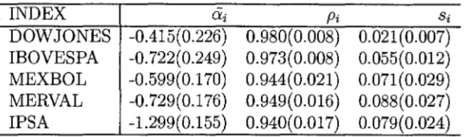
Univariate stochastic volatility mo deIs can be estimated under our methodology by simply assuming that k = O. Therefore, it is quite natural to begin with individual analysis for each particular country's returns series. We have used the same hyperparameter specifications (when needed) and simulation directives. Table 3 summarizes the results. It can be seen, for instance, that all series present highly persistent volatilities (Pi dose to unity).

INDEX ai Pi Si

DOWJONES -0.415(0.226) 0.980(0.008) 0.021(0.007) IBOVESPA -0.722(0.249) 0.973(0.008) 0.055(0.012) MEXBOL -0.599(0.170) 0.944(0.021) 0.071(0.029) MERVAL -0.729(0.176) 0.949(0.016) 0.088(0.027) IPSA -1.299(0.155) 0.940(0.017) 0.079(0.024)

Table 3: Univariate analyzes: retrospective posterior means and standard deviations (in parenthesis) for the stochastic volatility parameters.

Also, the series seem to have similar behavior with quite overlapping periods of high volatility, this being particularly emphasized by the Brazilian, Mexican and Argentinian indexes after August, 1997. In what follows we have applied our methodology to both one and two-factor stochastic volatility models.

3.3.2 One-factor stochastic volatility model

ai CPi U

-10.643(0.268) 0.965(0.012) 0.088(0.026)

INDEX

ã

i Pi Si

DOWJONES -0.739(0.235) 0.984(0.006) 0.011(0.004) IBOVESPA -1.463(0.203) 0.958(0.014) 0.084(0.027) MEXBOL -1.061(0.277) 0.985(0.011) 0.012(0.010) MERVAL -1.677(0.162) 0.910(0.028) 0.186(0.062) IPSA -1.464(0.097) 0.881(0.036) 0.134(0.048)

TabIe 4: One-factor model: retrospective posterior means and standard deviations (in paren-thesis) for the stochastic volatility parameters defining the common factor variance (upper)

and the specific variances (lower).

The factor Ioadings' posterior means in the one-factor mo deI is virtually the same as those obtained in the two-factor model (not presented here for the sake of space). This empiricaI evidence supports the argument that the first factor refiects the overall dependence of the time series through time. All other comparisons are similarly conclusive and suggest that the one-factor model fits well the dataset. Despite this fact, a two-factor stochastic volatility model has been fitted to the data in order to identify possible subtIeties overlooked by the one-factor model.

3.3.3 Two-factor stochastic volatility model

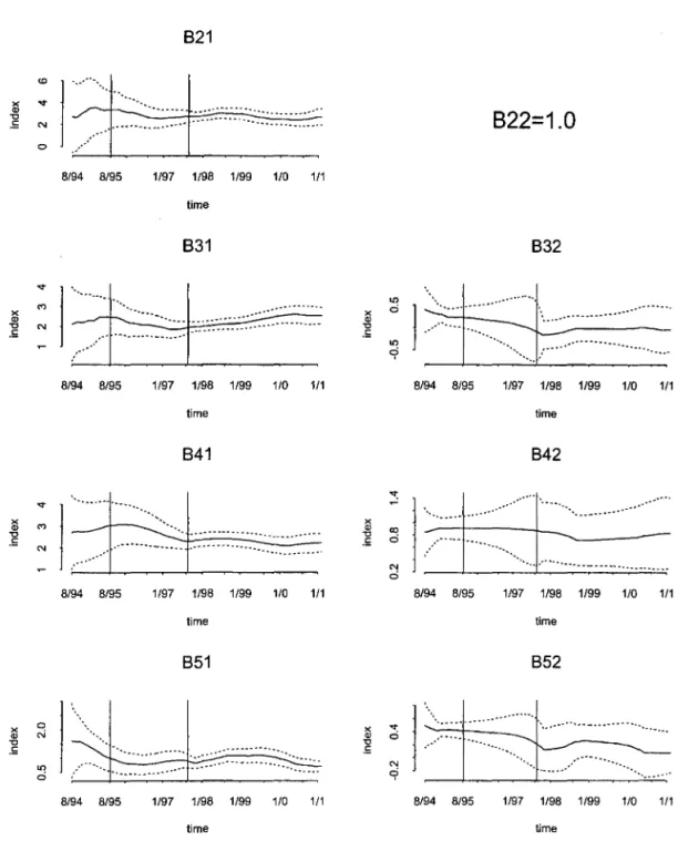
The following exhibit shows point estimates (posterior means) for the factor Ioadings, f3t for five time points.

9/9/95 10/29/96 12/2/97 1/12/99 2/1/2000

1.00 0.00 1.00 0.00 1.00 0.00 1.00 0.00 1.00 0.00

f3t= 3.39 1.00 2.57 1.00 _{2.47 0.91 2.02 0.90} 2.79 1.00 _{2.01 0.85} 3.00 1.00 _{2.18 0.71} 2.51 1.00 _{2.57 0.75} 0.22 0.96 0.11 0.81 -0.16 0.85 -0.03 1.08 -0.02 0.94 3.04 0.41 2.73 0.36 2.38 0.12 2.37 0.25 2.10 0.16

structures, common and specific, for all the indexes under consideration. The results are virtually the same when setting

Ro

=

0.001.

1 -10.201(0.416) 0.987(0.007) 2 -8.340(3.802) 0.997(0.002)

u

0.064(0.019) 0.972(0.022)

0.143(0.037) 0.346(0.106)

Table 5: Two-factor model: retrospective posterior means and standard deviations (in paren-thesis) for the stochastic volatility parameters defining the common factor variances.

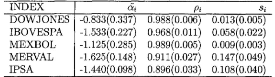
INDEX ai Pi Si

DOWJONES -0.833(0.337) 0.988(0.006) 0.013(0.005) IBOVESPA -1.533(0.227) 0.968(0.011) 0.058(0.022) MEXBOL -1.125(0.285) 0.989(0.005) 0.009(0.003) MERVAL -1.625(0.148) 0.911(0.027) 0.147(0.049) IPSA -1.440(0.098) 0.896(0.033) 0.108(0.040)

Table 6: Two-factor model: retrospective posterior means and standard deviations (in paren-thesis) for the stochastic volatility parameters defining the specific variances.

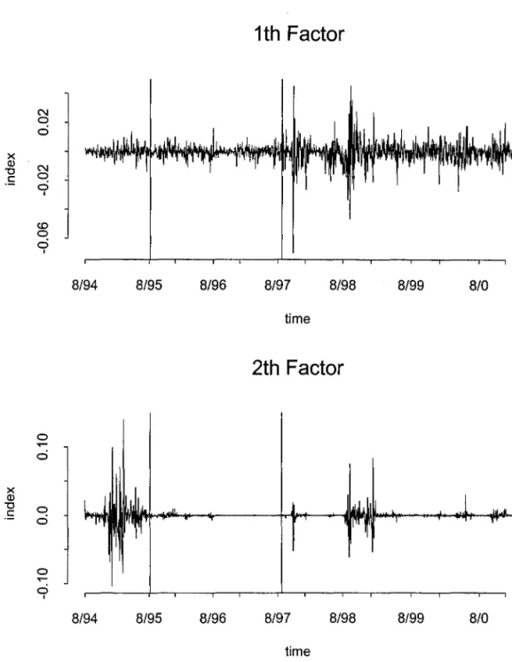
Graphical summaries are presented in Figures 2 to 4. Figure 2 shows the posterior means for the factor loadings through time and shows that there is little variation on the weights attributed to the factors across time. Figure 3 presents the posterior means for the common factors. It can be argued that the first common factor is virtually the stochastic component underlying the North American index, the Dow Jones. Analogously, the second common factor shows a behavior similar to those experienced by all four Latin American indexes. This latter factor, for instance, captures the highly volatile period that extends from earlier 1994 to late 1995.

Figure 4 presents the factorization of the returns' volatilities among the three factors: two common factor and the specific factor.

with the collapse of Thai Baht and Hong Kong dollar attack by speculators in October and

November, 1997, (iii) the Siberian Cold that took place in Russia in early August, 1998, and

finally (iv) the Brazilian Fever in January, 1999. This results corroborates with our earlier arguments about contagion. More specifically, there seems to exist contagion amongst Latin American countries.

It is worthwhile to mention that both one and two-factor models are able to capture the overall leveI of the time series volatilities, while their univariate counterparts are more erratic, refiecting their struggle to locate and estimate the series' stochastic volatility's leveIs (graph not presented).

4

Final comments and future work

In this article we have combined factor mo deIs with multivariate stochastic volatility models in order to learn and analyze the comovements amongst several Latin American stock price indexes. We have arguably shown that the time varying covariance structure could be modeled by one or two common factors and that some sort of contagion, as measured by abrupt changes in the time series correlations, was present in most ofthe series during periods of economical instability.

Using our methodology and the Bayesian approach it is fairly straightforward to compute predictives,

p(Yt+hIYt)

=

J

p(Yt+hl°t+h)P(°t+hIYt)d0t+h

with p( Ot+h IYt) accurately represented by the MCMC draws. Interesting by-product quanti-ties are E(Yt+h,íIYt+h,j, Yt) and V(Yt+h,íIYt+h,j, Yt) which assess the future (average) behaviour of a certain market, Yi, to shocks received by another market, Yj at a certain period of time. However, several interesting questions remain unanswered either because statistical method-ology is not available for meaningful and practical answers or because they need further and careful thought. Several of those questions are the following:

1. How to incorporate pre-specified structural changes (such as Markov switching regimes, for instance), in the series mean leveIs and variances?

2. Are there alternative ways of stochastically pinpointing periods of time where possible shifts have happened in the time series leveIs and/or volatilities without appealing for pre-specified structures?

BIBLIOGRAPHY

Agénon, P.R., Aizenman, J. and Hoffmaister, A. (1998) Contagion, bank lending spreads, and output fluctuations. Working paper, 6850. National Bureau of Economic Research.

Aguilar, Q. and West, M. (2000) Bayesian dynamic factor models and variance matrix discounting for portfolio allocation. Journal of Business and Economic Statistics (June 2000 Issue).

Bartholomew, D.J. (1995) Spearman and the origin and development of factor models.

British Journal of Mathematical and Statistical Psychology, 48, 211-220.

Diebold, F. X. and Nerlove, M. (1989) The dynamics of exchange rate volatility: A multi-variate latent factor ARCH model. Journal of Applied Econometrics, 4, 1-21.

Edwards, S. and Susmel, R. (2000) Interest rate volatility and contagion in emerging markets: evidence from the 1990s. Working paper. Anderson Gradutae School of Business, UCLA.

Engle, R. (1987) Multivarite ARCH with factor structures - cointegration in variance. Technical Report. University of California at San Diego.

Forbes, K. and Rigobon, R. (2000) Contagion in Latin America: definitions, measurement, and policy implications. Working paper, 7885. National Bureau of Economic Research.

Giakoumatos, S.G., Dellaportas, P. and D.D., Politis (1999) Bayesian analysis of some multivariate time-varying volatility models. Technical Report. Department of Statistics, Athens University of Economics and Business, Greece.

Harvey, A.C., Ruiz, E. and Shephard, N. (1994) Multivariate stochastic variance models.

Review of Economic Studies, 61, 247-264.

Jacquier, E., Polson, N.G. and Rossi, P. (1995) Models and priors for multivariate stochastic volatility. Discussion Paper. Graduate School of Business, University of Chicago.

Kim, S.N., Shephard, N. and Chib, S. (1998) Stochastic volatility: likelihood inference and comparison with ARCH models. Review of Economic Studies, 65, 361-393.

Lopes, H. F., Aguilar, O. and West, M. (2000) Time-varying covariance structures in currency markets. In Proceedings oi the XXII Brazilian Meeting of Econometrics.

Pitt, M.K. and Shephard, N. (1999) Time varying covariances: A factor stochastic volatility approach (with discussion). In Bayesian statistícs 6 (eds J.M. Bernardo, J.O. Berger, A.P. Dawid and A.F.M. Smith), pp. 547-570. London: Oxford University Press.

Rigobon, R. (1999) On the measurement of the international propagation of shocks. Working paper. Sloan School of Management, MIT.

Sentana, E. (1998) The reIation between conditionally heteroskedastic factor mo deIs and factor ARCH models. Econometrics Journal, 1, 1-9.

Shephard, N. (1996) StatisticaI aspects of ARCH and stochastic volatility. In Time Series

Models in Econometrics, Finance and Other Fields (eds D.R. Cox, D.V. HinkIey and O.E.

Barndorff-Nielsen). London: Chapman and Hall.

LOG(DOWJONES)

ｾ＠

ｾ＠

o

ｾ＠ oi

" '" oi

N

oi

8194 8195 6/96 8/97 8196 6/99 6/0

lime

LOG(IBOVESPA)

ＱＺＱｾ＠

8194 8195 6/96 8197 8198 8/99 8JO

time

LOG(MEXBOL)

o

ｾ＠

..

ｾ＠

oi 1: o

- oi

ｾ＠

"'

8f94 8/95 8/96 8/97 8198 8/99 8/0

lime

LOG(MERVAL)

ｾ＠

Ｚｾ＠

" o oi

'"

.,;

8/94 8195 8/96 8/97 8198 8199 810

time

LOG(IPSA)

8194 8(95 8/96 8/97 8198 8/99 8/0 ti"",

DIFF(LOG(DOWJONES))

11

ｾ＠

o

ｾ＠ 2l

ｾ＠

:g 9

8194 8/95 8/96 8/97 8196 8199 8/0

time

DIFF(LOG(IBOVESPA))

M

ｾｾｾＮｾ＠

ti

x ., ] o

ｾ＠

8194 8195 8196 8/97 8/98 6/99 6/0

time

DIFF(LOG(MEXBOL»

o

ｾ＠

ti

.8 ｾ＠ "

ｾ＠

'"

8194 8/95 6/96 8197 8198 8199 aIO

lime

DIFF(LOG(MERVAL))

8/94 8/95 8196 8/97 8/98 8/99 810

lime

DIFF(LOG(IPSA))

8/94 8/95 8/96 8/97 8198 8/99 810

time

x

{'l

.5 N o

...

N

...

N

o N

. "

Ó

821

l=J

" ... _--- -.... ----_._-... _----_ .. '.

ｾｮ＠ • • • • • • • • • •

==::::

...

8/94 8/95 1/97 1/98 1/99 1/0 1/1

time

831

8/94 8/95 1/97 1/98 1/99 1/0 1/1

time

841

ｾＺＺＺＺＺＺＺＺＺｾ＠

8/94 8/95 1/97 1/98 1/99 1/0 1/1

time

851

8/94 8/95 1/97 1/98 1/99 1/0 1/1

time

"

x

Q)

'"

"O _Ó .50

N

Ó

x ...

ｾ＠ o

.50

822=1.0

832

8/94 8/95 1/97 1/98 1/99 1/0 1/1

time

842

8/94 8/95 1/97 1/98 1/99 1/0 1/1

time

852

ｾﾷＺＺﾷﾷｴﾷﾷﾷﾷﾷﾷﾷﾷﾷﾷﾷｾ＠

- ' 0 " - •••••••..•

8/94 8/95 1/97 1/98 1/99 1/0 1/1

time

N o

o

x

Q)

N "O

.5: o

_o

I

co o

o

I

8/94

o

...

o

x

Q)

"O _o

.5:

_o

o

...

o

I

8/94

1th Factor

8/95 8/96 8/97 8/98 8/99

time

2th Factor

8/95 8/96 8/97 8/98 8/99

time

Figure 3: Common factors (posterior means).

8/0

DOWJONES DOWJONES DOWJONES

factar's weigth (1) factar's weigth (2) idiasyncratic's weight

::l

ｾ＠

ci ｾ＠ci

j _ci j ｾ＠ j _ci

ci

:; o o

ci ci

8194 8195 1/97 1198 1/99 1/0 1/1 8/94 8195 1/97 1/98 1/99 110 111 8/94 8/95 1197 1198 1/99 110 111

time lime lime

IBOVESPA IBOVESPA I BOVESPA

factar's weigth (1) factar's weigth (2) idiasyncratic's weight

ci ::l ｾ＠ci

i _ci j ｾ＠

i

_ci

" ci

o _:; o

ci ci

8/94 8195 1/97 1/98 1199 1/0 111 8194 8195 1197 1198 1/99 110 111 8194 8195 1/97 1198 1199 110 111

lime lime time

MEXBOL MEXBOL MEXBOL

factar's weigth (1) factar's weigth (2) idiasyncratic's weight

ｾ＠

::l ｾ＠

ci ci

i ｾ＠ _j

ｾ＠ ] ｾ＠ _ci

" ci ci

o o _:;

ci o

8194 al9S 1197 1198 1/99 110 111 8/94 8195 1197 1198 1/99 1/0 111 8194 8195 1197 1198 1199 110 111

lime lime time

MERVAL MERVAL MERVAL

factar's weigth (1) factar's weigth (2) idiasyncratic's weight

::l

ｾ＠

ｾ＠

tJL

ｾ＠

o ci

I

ci

i

:; j ci

o o o

o o ci

8194 8195 1/97 1198 1/99 110 111 8/94 8/95 1/97 1/98 1/99 110 111 8/94 8195 1/97 1198 1/99 110 111

time time time

IPSA IPSA IPSA

factar's weigth (1) factar's weigth (2) idiasyncratic's weight

ｾ＠

ｾ＠

ｾ＠ ｾ＠

ci ci ci

.- :; j j ｾ＠

ci ci

o o

.,

o

.,

8194 8/95 1/97 1/98 1/99 110 111 8/94 8195 1/97 1/98 1/99 110 111 8/94 8/95 1197 1/98 1199 110 111

time time time

'" '" o o '" '" O "

ｾ＠

O U = ó ó o Ó ó Ó o Ó = ó Ó o Ó o o

Bl94 8/95 8196

8/94 8/95 8/96

8/94 8/95 8196

8/94 8/95 BI"

8/94 8195 8196

corr(Yl, Y2IK=1)

8197 8/98 8/99

lime

corr(Yl,Y4IK=1)

8/97 8/98 8/99

time

corr(Y2,Y3IK=1)

8/97 8/98 BIS9

lime

corr(Y2, Y5IK=1)

8197 Bl98 _BI"

time

corr(Y3,Y5IK=1)

8/97 8/98 8/99

time

corr(Yl, Y3IK=1)

8/0 8/94 8/95 6196 8/97 8/98 Bl99 8/0

time

corr(Yl,Y5IK=1)

8/0 8/94 8/95 8/96 8/97 8/98 8/99 BlO

lime

corr(Y2,Y4IK=1)

BlO 8/94 a!9S 8/96 8/97 8/98 8/99 8/0

lime

corr(Y3,Y4IK=1)

8/0 8/94 8195 8/96 8/97 819B 8/99 8/0

time

corr(Y4,Y5IK=1)

6/0 8/94 8195 8196 Bl97 B/9B 8/99 8/0

time

Figure 5: Posterior mean of time series correlations. Pairs of verticallines represent the first and last business days of the following months: 12/94,10-11/97,8/98 and 01/99.

• • • • • • • • • • • _ . . . I . . . I li . , .