Computational Statistics and Data Analysis

Contents lists available atScienceDirect

Computational Statistics and Data Analysis

journal homepage:www.elsevier.com/locate/csda

Surveillance to detect emerging space–time clusters

Renato Assunção

a,∗

, Thais Correa

b

a_{Departamento de Estatística, Universidade Federal de Minas Gerais, 31270-901 Belo Horizonte, MG, Brazil} b_{Departamento de Matemática, Universidade Federal de Ouro Preto, Brazil}

a r t i c l e i n f o

Article history:

Available online 5 November 2008

a b s t r a c t

The interest is on monitoring incoming space–time events to detect an emergent space–time cluster as early as possible. Assume that point process events are continuously recorded in space and time. In a certain unknown moment, a small localized cluster of increased intensity starts to emerge. Its location is also unknown. The aim is to let an alarm to go off as soon as possible after its emergence, but avoiding that it goes off unnecessarily. The alarm system should also provide an estimate of the cluster location. In addition to that, the alarm system should take into account the purely spatial and the purely temporal heterogeneity, which are not specified by the user. A space–time surveillance system with these characteristics using a martingale approach to derive the surveillance system properties is proposed. The average run length for the situation when there are clusters present in the data is appropriately defined and the method is illustrated in practice. The algorithm is implemented in a freely available stand-alone software and it is also a feature in a freely available GIS system.

©2008 Elsevier B.V. All rights reserved.

1. Introduction

The ongoing and systematic collection of data, as well as its analysis, became essential long ago to the planning, implementation, and evaluation of public health practice. However, as more and more health data are stored in electronic form in a timely way, it is increasing the need for methods which can detect quickly anomalies in a continuously updated database, with minimum input requirements from users. Currently, early disease outbreak detection systems are the object of intense demand by government agencies, specially public health departments. One reason for this heightened interest on the subject is the threat of bioterrorism (Buehler et al.,2004;Henderson,1999), but these systems have a much larger and much older application scope. In fact, early outbreak detection methods have always been a matter of concern to public health (Hardy, 2001). In the new context of spatially referenced data, these methods face important analytical challenges that include dealing with the adjustment for natural temporal and spatial variation, the unknown time, place and size of an emergent cluster, detecting an outbreak as early as possible, and the lack of suitable population-at-risk data.

Most statistical methods in use for the early detection of disease outbreaks are purely temporal in nature (Sonesson and Bock, 2003;Höhle,2007;Höhle and Paul, 2008). Hence, they are usually applied to monitor data from large area regions without concern to their geographical location within the monitored regions. They lack power to detect outbreaks that start locally since the affected areas are submerged into large regions with usual incidence rates. One possible solution is to partition the large region into small areas and to apply the purely temporal methods in each small area separately and in parallel. However, this procedure leads to a severe problem of multiple testing, generating many more false signals than the nominal statistical significance level indicate. As a consequence, these purely temporal methods are not appropriate when the data are collected with space and time information. In addition to these problems, there is the expectation that using

∗_{Corresponding author. Tel.: +55 31 3409 5940; fax: +55 31 3409 5924.} E-mail address:[email protected](R. Assunção).

0167-9473/$ – see front matter©2008 Elsevier B.V. All rights reserved.

the now readily available spatial information can facilitate the detection and localization of emergent clusters (Buckeridge et al., 2005).

The primary purpose of this paper is to suggest a method for the quick detection of space–time emergent clusters in a set of point process events. The requirements to establish a surveillance system, either accounting for spatial structure or not, are generally structured around a basic trade-off: the need for quickly detecting possible outbreaks must be balanced against the need to avoid a high rate of false alarm signals. Our method allows the user to control these trade-off elements in a simple way.

We introduce a stochastic model to describe eventually emerging spatial clusters with minimum requirement of user-defined parameters. When there are no clusters, we assume that the events’ density is separable, meaning that it is the product of arbitrary spatial and temporal functions. More importantly, our method does not require the functional specification of these purely spatial or the purely temporal functions. As an alternative to this model, we assume that somewhere, at some moment, one or more space–time high intensity clusters start to emerge. We develop a likelihood model for this pair of hypotheses and monitor the incoming events with a spatial version of the Shyriaev-Roberts statistic. The Shiryaev–Roberts statistic is well known on industrial statistics applications but it is not so common in biometrical work. We use the martingale structure of the Shiryaev–Roberts statistic to derive the values for the tuning parameters of our method.

The next section contains a brief review of the prospective space–time methods available and introduces the main definitions and notation used in the paper. In Section3, we present our proposal using the Shiryayev-Roberts control chart method based on martingales. Section4presents an analysis of the impact of tuning parameters. In Section5we show the results of a Monte Carlo study of the method performance. For this, we need to define appropriately what is the expected time until detection when there are clusters present in the data. We are specially interested in the effects of the tuning parameters in our method performance. Section6illustrates the use of the method to detect and to identify the particular events that are associated with the space–time clusters. We use the classic Burkitt’s lymphoma dataset (Williams et al., 1978) and a Brazilian dataset of Meningitis cases in three years of observation. We analyzed the data using a freely available stand-alone software where our method is implemented. Finally, we close in Section7with a discussion and a summary of the main conclusions.

2. Prospective space–time surveillance for localized clusters

The traditional methods for space–time cluster detection are retrospective in nature. That is, they search in a database of past events for evidence of presence of space–time clusters. In contrast, our interest is on prospective methods for geographically restricted: an events’ database is updated regularly and then an algorithm should run to help deciding on the emergence of localized space–time clusters. Hence, the clusters must be alive, in the sense that at least some of the most recent events belong to the eventually detected clusters. The regularly updating nature of the database brings two difficult problems. In the first place, the possibility of using too many significance tests as, for example, if one statistical test is carried out every time the database is updated. This induces a severe multiple testing problem with too many false alarms for clusters. As a consequence, such a method would be soon discredited as unreliable. In the second place, reducing in some way the false alarm rate could imply in a long delay to signal a truly emerging space–time cluster. The trade-off between these two problems must be explicitly recognized in any methodology.

A thorough literature review can be found in the book edited byLawson and Kleinman(2005), inSonesson and Bock

(2003), and inWaller and Gotway(2004). We give here a brief overview of the main proposals. There are non-spatial, purely temporal methods derived from quality control ideas concerned with the monitoring of a stochastic process in time. The Shewart Chart Control is a very simple and popular method but it is not sensitive to small changes in the process. The Cumulative Sum (CUSUM) method accumulates the recent evidence to the previous data until a certain threshold is crossed. It is better than Shewart to detect small changes in the purely temporal process and it has been shown that it has optimal properties in very simple scenarios (seeFrisén(2003)). Exponentially weighted moving average also accumulates evidence, as the CUSUM method, but it discounts observations as they get old (Frisén, 2003). All these methods assume that data are independent in time, which is not a realistic assumption in many applications.Kenett and Pollak(1996) uses Shiryaev–Roberts statistics to allow for dependent data. We review this work later in this section.

There are few space–time oriented proposals. One recent promising method has been suggested byKulldorff(2001) who used a space–time scan statistic for area data. The main difficulty is the control of overall significance level for a sequence of periodic tests, although each individual test has error type I adjusted for all previous analysis at each time moment. We discuss this issue in more detail in the last section.

Rogerson (2001) suggested a statistic based on local Knox statistic that requires only cases data in the form of a space–time point process.Marshall et al.(2007) found severe problems with the probability approximations used in this methods, suggesting that it should not be used.Marshall et al.(2007) demonstrate that the ARL performance of the Rogerson method is highly influenced by some required threshold values, by the population density, and by the region shape. As a consequence, the nominal performance measures associated with Rogerson method are not valid and this makes impossible the tuning of the method without computer simulation.

likelihood ratio test statistic scanning over all possible cylinders as clusters candidates. This method does not control overall error type I level for the sequence of periodic analysis.Diggle et al.(2005) andRodeiro and Lawson(2006) proposed a Bayesian method to model the space–time evolution of the incidence rate and to monitor for changes.

We base our proposal in the Shiryaev–Roberts (SR) surveillance method that was developed only for temporal processes (Shiryaev,1963;Roberts,1966;Kenett and Pollak, 1996). Suppose that a sequence of possibly dependent random variables

X1

,

X2

, . . .

is observed. Two possible models are considered. In one, a sudden change in the stochastic process occurs at the

unknown momentkandfk

(

x1

,

x2

, . . .

xt

)

is the joint density distribution of the firsttrandom variables. In the second model,

no change ever occurs. In this case, we assume thatk

= ∞

and writef∞

(

x1

,

x2

, . . .

xt

)

for the joint density. Any surveillance

method implies a stopping timeT, the first moment when the alarm goes off. LetEk

(

·

)

be the expectation with respect to fk. The meanE∞

(

T

)

is called theAverage Run Lengthand it is denoted byARL0. Clearly, it is desirable to makeARL0large.

Typically, the user establishes an acceptable minimum thresholdBfor this parameter. That is, we wantARL0

₌

_E

∞

(

T

) >

B,

whereBis known.

One approach would be to maximize the likelihood ratio over all possible values of the unknown parameterkdefining the statistic

max

1≤k≤t

fk

(

X1

, . . . ,

Xt

)

f∞

(

X1

, . . . ,

Xt

)

.

Rather than adopting this approach, the Shiryaev–Roberts statisticRtuses the sum of likelihood ratiosfk

/

f∞for all possible

change-point momentsk:

Rt

=

t

X

k=1

f(k)

(

X1

,

X2

, . . . ,

Xt

)

f∞

(

X1

,

X2

, . . . ,

Xt

)

.

The alarm goes off ifRtis too large, that is, ifRt

≥

A. The stopping timeTAis defined as

TA

=

min

{

t

|

Rt

≥

A

}

.

It remains to findAsuch thatARL0

₌

_E

∞

(

TA

) >

B.

Following the notation ofKenett and Pollak(1996), underP∞, the sequence

Λk,t

=

fk

(

X1

,

X2

, . . . ,

Xt

)

f∞

(

X1

,

X2

, . . . ,

Xt

)

is a martingale with expected value equal to 1, even with dependent observations. Therefore,

Rt

−

t

=

t

X

k=1

(

Λk,t

−

1

)

is a zero mean martingale. By the Optional Sampling Theorem, we have

E∞

(

RTA

−

TA

)

=

0

,

and therefore

E∞

(

TA

)

=

E∞

(

RTA

).

By definition,RTA

≥

Aand henceE∞

(

TA

)

≥

A. Therefore, takingA

=

Bsatisfies the conditionE∞

(

NB

)

≥

B.

There are several advantages associated with the Shiryaev–Roberts method in the time series context. First, it can be shown that it exhibits some optimal properties in some simple scenarios (Pollak, 1985).Pollak(1985) proved that the Shiryaev–Roberts procedure is asymptotically (asB

→ ∞

) optimal in the sense of minimizing the supremum average delay to detection

sup

k≥1

Ek

(

T

−

k

|

T

≥

k

)

over all stopping timesTthat satisfyE∞

(

T

)

≥

B.Yakir(1994) found that this procedure is strictly optimal for the problem

of minimizing the average run length to detection over all stopping timesTthat satisfyE∞

(

T

)

≥

BwhenX1

,

X2

, . . . ,

Xk−1

are iid random variables. Furthermore, in terms of the delay time for the alarm going off after the purely temporal clusters starts to emerge, the Shiryaev–Roberts and the usual CUSUM method are similar (Shiryaev,1963;Roberts,1966;Pollak and Siegmund, 1985;Mevorach and Pollak, 1991). The Shiryaev–Roberts method does not require independence between observations. It can also be shown that Shiryaev–Roberts is at least as efficient as some optimal classical procedures (Kenett and Pollak, 1996).

One difficulty to use the Shiryaev–Roberts method is that it depends on the complete specification of the joint distribution ofX1

, . . . ,

Xn after a change occurs atk. This is not simple to be done in the purely temporal context and the difficulty

3. Detection of emerging space–time clusters

3.1. A model for emerging clusters

LetNbe a Poisson process inR3partially observed in the three-dimensional regionA

×

(

0

,

T

]

.

The events

(

si

,

ti

)

=

(

xi

,

yi

,

ti

)

are indexed byi

=

1

,

2

, . . .

, and we assume thatt1

<

t2

<

· · ·

. LetN

(

C

)

be the number

of events in the setC

⊂

A

×

(

0

,

T

]

. We haveN

(

C

)

distributed as a Poisson random variable with mean

µ(

C

)

given by the integral of the intensity function

λ(

x

,

y

,

t

)

≥

0 overC:

µ(

C

)

=

Z

C

λ(

x

,

y

,

t

)

dxdydt

.

A special type of setCis a cylinder given byC

=

B

(

s

, ρ)

×

(

ta

,

tb]whereB

(

s

, ρ)

is the disc centered ats

=

(

x

,

y

)

∈

A

with radius

ρ

, andta

<

tb.

Let

µ

=

µ(

A

_×

₍

₀

_,

T

_]

₎

_{be the expected number of events in the observation region and define the marginal spatial and}

temporal densities by

λ

S

(

x

,

y

)

=

µ

−1

Z

(0,T]

λ(

x

,

y

,

t

)

dt

,

and

λ

T

(

t

)

=

µ

−1

Z

A

λ(

x

,

y

,

t

)

dxdy

,

respectively. Note that

Z

A

λ

S

(

x

,

y

)

dxdy

=

Z

(0,T]

λ

T

(

t

)

dt

=

1

.

Given that an event

(

s

,

t

)

occurred inA

×

(

0

,

T

]

, the functions

λ

S

(

x

,

y

)

and

λ

T

(

t

)

represent the probability density ofsand

t, respectively.

We define now the pair of situations we will consider. The first one is that without space–time clusters. In this case, we have a separable intensity

λ(

x

,

y

,

t

)

=

µ λ

S

(

x

,

y

) λ

T

(

t

)

where

λ

_S

(

x

,

y

)

and

λ

T

(

t

)

are arbitrary and unspecified. That is, they

are nuisance parameters.

The alternative situation assumes that there exists a time

τ

, a constant

ε >

0, and a cylinderC

=

B

(

s

, ρ)

×

(

ta

,

tb

]

(yet

to be defined) such that

λ(

x

,

y

,

t

)

=

µ λ

S

(

x

,

y

) λ

T

(

t

) (

1

+

ε

IC

(

x

,

y

,

t

)).

This intensity function can not be written as a product of two functions, one depending only in space and the other only in time. The parameter

ε

is the relative change on the events intensity within the cluster and it must be specified by the user.

Assunção and Maia(2007) andAssunção et al.(2007) used a similar pair of alternative models in the context of space–time point process data.

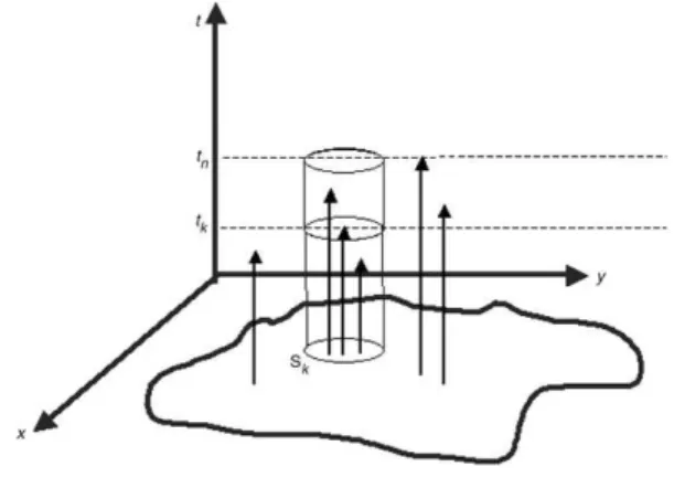
To define a useful class of cylindersC, we start considering that, if a higher incidence cluster emerges, we must be able to detect it through the observed events. That is, non-events (or void spaces) do not bring information about an emerging cluster. Hence, we decided to constraintato be equal to one of the observed events timestk. Additionally, the cylinders

should be centered around its corresponding spatial locationsk. Since the interest is only on alive clusters, the endpointtb

is equal to the timetnof the current last observed event. That is, we consider cylinders of the formB

(

sk

, ρ)

×

(

tk

,

tn

]

, with k

<

n, where

(

sk

,

tk

)

is one previously observed event while

(

sn

,

tn

)

is the last observed event at a given moment. The disc B

(

sk

, ρ)

has a radius

ρ

specified by the user. To simplify notation, we denote byCk,nthe cylinderB

(

sk

, ρ)

×

(

tk

,

tn]with k

<

n. We extend the notation to include the casek

=

n, writingCn,nto represent the null set.

3.2. A sequential procedure to detect emerging clusters

To define a statistic, we consider the likelihood of the space–time Poisson processes whennevents have been observed. If no cluster is emerging, we have

L∞

=

n

Y

i=1

λ(

xi

,

yi

,

ti

)

!

exp

−

Z

R3

λ(

x

,

y

,

t

)

dxdydt

.

Under the alternative scenario that a cluster started emerging at timetk

<

tn, we have

Lk

=

n

Y

i=1

λ(

xi

,

yi

,

ti

) (

1

+

ε

ICk,n

(

xi

,

yi

,

ti

))

!

exp

−

Z

R3

λ(

x

,

y

,

t

)

dxdydt

exp

−

ε

Z

Ck,n

λ(

x

,

y

,

t

)

dxdydt

!

,

Therefore, a space–time version of the SR test statisticRnbecomes

Rn

=

n

X

k=1

Lk L∞

=

n

X

k=1

("

_n

Y

i=1

(

1

+

ε)

ICk,n

(

xi

,

yi

,

ti

)

#

exp

−

ε

Z

Ck,n

λ(

x

,

y

,

t

)

dxdydt

!)

=

n

X

k=1

(

1

+

ε)

N(Ck,n) _exp

₍

₋

_{ε µ(}

_C

k,n

))

(1)

=

n

X

k=1

Λk,n

.

(2)

The expressionΛk,ncan be seen as a contrast between the observed numberN

(

Ck,n

)

of events inCk,nand its expected value

under the no-cluster situation. In fact, if

ε

is small,

Λk,n

≈

(

1

+

ε)

N(Ck,n)

(

1

−

ε)

µ(Ck,n)

≈

1

+

ε

N

(

Ck,n

)

−

µ(

Ck,n

)

.

The parameter

ε >

0 is known (user-specified) and measures the anticipated relative change in the events’ density. Note that

Λn,n

=

(

1

+

ε)

N(Cn,n,)exp

(

−

εµ(

Cn,n

))

=

(

1

+

ε)

0exp

(

0

)

=

1

.

Our surveillance method calculatesRnas then-th event arrives, substituting the unknown

µ(

Ck,n

)

by an estimate

µ(

ˆ

Ck,n

)

.

The estimation of

µ(

Ck,n

)

is discussed in Section3.3. The alarm goes off whenRn

≥

Afor the first time.

In summary, the algorithm associated with our proposal requires as input:

•

a set ofncase events, specified by their spatial coordinatesx,yand timet;

•

the value of three user-specified tuning parameters:

. the anticipated relative change

ε

in the density within the cluster; . the anticipated radius

ρ

for the cluster;

. the thresholdA, which should be approximately equal to the desiredARL0_.

Iteratively inn, we calculateRn. The output is a sequence of valuesRnwherenis the number of events. IfRn

>

Afor any n, the alarm goes off.

If the alarm goes off, one important practical issue is the space–time cluster location. Suppose that the alarm goes off at then-th event. That is,Rt

≥

Afor the first time att

=

n. Since

Rn

=

n

X

k=1

Λk,n

=

Λ1,n

+

Λ2,n

+

. . .

Λn,n

.

The large values ofΛk,nare those contributing to the alarm triggering. LetΛk∗,n

=

max

{Λk

,n

,

1

≤

k

≤

n

}

. A cluster estimate

is built by taking the spatial coordinates

(

xk∗

,

yk∗

)

of thek

∗

-th event as the center of the cylinder basis, and by taking its height equal to

[

tk

∗

,

tn

]

. That is,Ck∗_,nis the space–time cluster estimate.

3.3. Estimation of

µ(

Ck,n

)

Typically, the user will not be able to specify the purely spatial

λ

S

(

x

,

y

)

and the purely temporal

λ

T

(

t

)

functions. Therefore,

it is relevant in practice to alleviate him from such requirements. Rather than using the mean

µ(

Ck,n

)

in(1), we use the data

themselves to estimate it. From the non-homogeneous Poisson process properties, under the null hypothesis, fork

<

nwe have:

µ(

Ck,n

)

=

Z

Ck,n

λ(

x

,

y

,

t

)

dxdydt

=

µ

Z

B(sk,ρ)

λ

S

(

x

,

y

)

dxdy

Z

(tk,tn]

λ

T

(

t

)

dt

.

Therefore, an estimate of

µ(

Ck,n

)

under the hypothesis that there are no clusters is given by

ˆ

µ(

Ck,n

)

=

N

(

B

(

sk

, ρ)

×

(

0

,

tn

]

)

N

(

A

×

(

tk

,

tn

]

)

n

,

whereN

(

B

(

sk

, ρ)

×

(

0

,

tn]

)

is the number of events within the discB

(

sk

, ρ)

irrespective of occurrence time,N

(

A

×

(

tk

,

tn]

)

is the number of events between timestkandtn, irrespective of their spatial location, andnis the total number of events at

Fig. 1. The estimateµ(Cˆ k,n).

3.4. Iterative calculation of Rn

Every new event requires the recalculation of allnterms in(2). We can decrease substantially the amount of numerical calculations by means of an iterative procedure. Fork

<

n, letIk,n

=

I

(

k

sn

−

sk

k ≤

ρ)

. We have

N

(

Ck,n+1

)

=

N

(

Ck,n

)

+

Ik,n+1

and

µ(

Ck,n+1

)

=

µ(

Ck,n

)

+

µ (

B

(

sk

, ρ)

×

(

tn

,

tn+1

]

) .

Therefore, sinceΛ1,1

=

1, we can write recursively fork

<

n

+

1,

Λk,n+1

=

Λk,n

(

1

+

ǫ)

Ik,n+1 exp

(

−

ǫµ (

B

(

sk

, ρ)

×

(

tn

,

tn+1

]

)) .

By definition,Λn+1,n+1

=

1 and this completes the recursion.

In practice, to run the procedure, we need

µ(

ˆ

Ck,n+1

)

, rather than

µ(

Ck,n+1

)

. However, this estimated term can also be

calculated iteratively fork

<

n

+

1:

ˆ

µ(

Ck,n+1

)

=

1

n

+

1N

(

B

(

sk

, ρ)

×

(

0

,

tn+1

]

)

N

(

A

×

(

tk

,

tn+1

]

)

=

n

+

1

−

k

n

+

1 N

(

B

(

sk

, ρ)

×

(

0

,

tn

]

)

+

Ik,n+1

=

n n

+

1

n

−

k

+

1

n

−

k

µ(

ˆ

Ck,n

)

+

n

+

1

−

k n

+

1 Ik,n+1

= ˆ

µ(

Ck,n

)

+

k

(

n

+

1

)(

n

−

k

)

µ(

ˆ

Ck,n

)

+

n

+

1

−

k n

+

1 Ik,n+1

.

Fork

<

n

+

1, we can write

ˆ

Λk,n+1

=

(

1

+

ε)

N(Ck,n)+Ik,n+1exp

−

ε

Jn,k

+ ˆ

Λn+1,n+1

,

where

Jn,k

=

n

(

n

−

k

+

1

)

(

n

+

1

)(

n

−

k

)

µ(

ˆ

Ck,n

)

+

n

+

1

−

k n

+

1 Ik,n+1

.

Therefore,

Rn+1

=

n+1

X

k=1

ˆ

Λk,n+1

=

1

+

n

X

k=1

ˆ

Λk,n exp

₋

ε

k

(

n

+

1

)(

n

−

k

)

µ(

ˆ

Ck,n

)

Lε,n,k

,

where

Lε,n,k

=

(

1

+

ε)

exp

−

ε

n

+

1

−

k

n

+

1

Ik,n+1

.

We let 1

=

Λn+1,n+1

= ˆ

Λn+1,n+1. As a consequence, we obtainRn+1simply by updating the values ofΛk

ˆ

,nwith a few

4. Choice of tuning parameters

The variance of the test statisticRn

=

P

kΛk,nincreases with

ε

when we have no clusters. More importantly, the

distribution ofRnis quite asymmetric. Indeed, for one side a large negative deviate ofN

(

Ck,n

)

from its mean

µ(

Ck,n

)

pushΛk,n

towards its lower bound, equal to zero. For the other side, increasing a large positive deviate drivesΛk,ntowards infinity.

As a consequence, the false alarm rate increases with

ε

. The simulations in Section5will show these effects of changing

ε

on the surveillance system performance. Although analytical results are difficult to obtain, simple approximations provide some insight into this trade-off.

When there is no cluster emerging, we haveE

(

Λk,n

)

=

1 for all

ε

because E

(

Λk,n

|

H0

)

=

exp

(

−

ε µ(

Ck,n

))

E

[

(

1

+

ε)

N(Ck,n)

]

=

exp

(

−

ε µ(

Ck,n

))

exp

(µ(

Ck,n

)(

1

+

ε))

exp

(

−

µ(

Ck,n

))

=

1

.

Then,E

(

Rn

)

=

nfor all

ε

, as we could expect from the martingale approach of Section2.

Suppose now that a cluster emerges and thatN

(

Ck,n

)

∼

Poisson

(µ(

Ck,n

) (

1

+

ε

∗

))

. At this point, we distinguish the true

rel-ative change

ε

∗from the one specified by the method (

ε

). They do not need to coincide. In this alternative situation we have

E

(

Λk,n

)

=

exp

(

−

ε µ(

Ck,n

))

E

[

(

1

+

ε)

N(Ck,n)

]

=

exp

(

−

ε µ(

Ck,n

))

exp

[

µ(

Ck,n

)(

1

+

ε

∗

)(

1

+

ε

−

1

)

]

=

exp

[

µ(

Ck,n

)εε

∗

]

>

1

.

That is,E

(

Λk,n

)

increases with

ε

(and with

ε

∗).

Therefore, apparently, the choice of

ε

does not affectRnwhen there is no cluster. When a cluster emerges, choosing a

large

ε

∗will increaseRnand speed up the threshold crossing, as we wish in this case. Hence, it seems that taking

ε

→ ∞

is

the a good strategy.

However, there is a penalty for choosing

ε

∗too large in that the Var

(

Λk,n

)

increases with

ε

∗when there is no cluster. In

fact,

Var

(

Λk,n

)

=

Var

[

exp

(

−

ε

∗

µ(

Ck,n

)) (

1

+

ε

∗

)

N(Ck,n)

]

which is equal to

exp

(

−

2

ε

∗

µ(

Ck,n

))

{

exp

(µ(

Ck,n

)((

1

+

ε

∗

)

2

−

1

))

−

exp

(

2

µ(

Ck,n

)(

1

+

ε

∗

−

1

))

}

.

This reduces to

exp

(µ(

Ck,n

)ε

∗2

)

−

1

→ ∞

,

as

ε

∗

→ ∞

.

Ultimately, this will increase the false alarm rate. Under no cluster, increasing

ε

∗too much implies in a larger variability ofRn. This is so, because the pairs of termsΛk,nare either uncorrelated (if the corresponding cylinders are non-intersecting)

or positively correlated (with correlation proportional of the intersecting volume). As a consequence, the variance of the stopping timeTAincreases as well as the probability thatRTAcrosses the thresholdAat a very early moment, as well as

much later than the expectedE

(

TA

)

=

A. Hence, there is a larger probability that the threshold will be crossed before any

cluster emergence. These effects will be clear in the simulations of Section5.

As shown in the simulations, changing the radius produces small effects on the surveillance system performance.

5. Method performance

We evaluated the performance of our method with Monte Carlo simulation using three types of scenarios. In the first type, there were no clusters and the purpose is to evaluate if the approximationA

=

B

≈

ARL0_{is appropriate. The geographical}

region was the rectangle

[

0

,

10

] × [

0

,

10

]

and the spatial location of an event was obtained by independently and uniformly generating coordinates on the square. Times between events were modelled by independent exponential random variables with mean equal to 1. Times and locations were independently generated and hence

λ(

x

,

y

,

t

)

=

0

.

01. The events were generated sequentially until the alarm was triggered.

In the second type of scenario, in addition to the events generated as in the first scenario, we also simulated events within a cylindrical cluster that emerged at some moment. The purpose of this second type of scenario is to evaluate the detection performance and the effects of the user-specified tuning parameters of our method. The cluster had the square basis

[

4

,

5

] × [

4

,

5

]

. It was kept alive from its outbreak until the alarm went off. We selected three different times for the cluster outbreak. In one case, the cluster starts at the beginning of the time period (whent

=

50) and we label this ascase B. In the second case, the cluster starts in the middle of the time period, whent

=

150, and this is labelledcase M. Finally, in the third case, the cylinder cluster starts late, att

=

300, and we labelled this ascase L.

Fig. 2. Scenario without cluster. The plots show the estimatedARL0_=E(T

A), the average number of events observed before a false signal is issued, versus the threshold limitA. Each curve corresponds to a value ofε. In all cases, we usedρ=1.

We will call this second type of scenario the homogeneous scenario because there is no spatial variation in the events’ intensity except that due to the cluster emergence. The third type of scenario was generated in the same way as the second type except by the use of a spatially heterogeneous density of the events locations. In this third scenario type, the spatial coordinates were generated using a mixture of four bivariate normal distributions. Therefore, at any time, some regions were more likely to observe an event than other regions.

We generated 1000 independent replications of each scenario. To run the surveillance procedure, we used several values for

ε

: 0

.

1

,

0

.

2

,

0

.

4

,

0

.

5

,

2

.

5

,

5

,

10

,

20. Note that, for the scenario without clusters, the true value of this parameter is zero, while in the scenarios with clusters, it is equal to 0

.

2.

No comparison with the scan statistic method fromKulldorff(2001) has been attempted because it takes too long to run. In each scenario, for a single simulated space time dataset with 1000 events, Kulldorff’s method takes 2 h and 26 min in a machine with 1.66 GHz and 1 Gb RAM when we ask for 999 Monte Carlo replications. To repeat this procedure for all the simulated datasets over the many scenarios is unfeasible.

5.1. Scenario without clusters

We used the values 50, 100, 200, 300, 400, and 500 for the threshold limitAand

ρ

=

1 for the spatial radius of the presumed cluster. If there are no clusters, any surveillance signal is a false signal. If the time period goes to infinity, the statisticRnwill cross the thresholdAwith probability one, irrespective of the presence of a real cluster. It is expected that,

in a fixed time period, the number of events until the alarm goes off increases with the increase of the thresholdA. If the approximationA

=

Bis reasonable, we should haveA

≈

ARL0_.

The graph inFig. 2shows in the vertical axis the estimatedARL0_{, the average number of events observed before a false}

signal is issued, versus the threshold limitAin the horizontal axis. The dashed line represents the lineARL0

=

A. The other lines represent the test results for different values of

ε

.

As we expect,ARL0_{increases with the thresholdA. For}

_ε

₌

₀

_.

_{1 and 0}

_.

_{2, the approximationARL}0

₌

_{Ais very good. For}

other values of

ε

this approximation deteriorates with the increase ofA. Initially, the departure from the lineARL0

₌

_Ais

larger the greater is

ε

. For example, whenA

=

500 and

ε

=

0

.

5, the estimatedARL0_{is 33% larger than the nominal value of}

500. However, the difference between the nominal valueAand the trueARL0_{does not increase monotonically with}

_ε

_{. With}

ε

≥

10, this difference is almost null. Setting

ε

≥

10 is an extreme choice since it means an emerging cluster with intensity 10 times larger than the baseline intensity. It is unlikely that our method is envisioned for such type of anticipated changes. This result shows that, when no cluster is present and within practical bounds for the expected relative change in intensity, selecting larger values for the user-specified

ε

parameter leads to conservativeARL0_{. That is, if the user is unsure}

about

ε

, selecting a larger value leads to longerARL0_{times than the nominal valueA.}

However, there is a trade-off in selecting

ε

too large in that the false alarm rate can increase, as we show in the next section. The reason for this behavior is the increase on the standard deviation of the stopping timeTAwith the increase of

ε

.Table 1shows this standard deviation for different choices of

ε

and thresholdA. The larger variability will increase the chances of observing much earlier and much laterTAthan its expected value. This increases the chance that an unmotivated

alarm sounds off before any cluster emerges. This behavior can be fully understood after we present the results of simulations with clusters.

5.2. Scenarios with clusters

Table 1

Standard deviation of the stopping timeTAfor different choices of thresholdAandε. In all cases we usedρ=1.

Threshold ε=0.1 ε=0.2 ε=0.4 ε=0.5 ε=2.5 ε=5 ε=10 ε=20

50 0.498 0.518 0.928 1.143 7.115 12.610 17.473 23.009

100 0.561 0.996 1.933 2.483 26.050 39.971 40.410 40.037

200 1.051 2.088 4.746 6.630 95.582 103.240 96.583 97.584

300 1.565 3.291 8.851 13.663 180.976 178.143 142.034 163.956

400 2.137 4.647 15.484 26.544 254.284 233.516 196.761 210.668

500 2.982 6.915 25.488 48.344 294.398 283.244 239.812 254.411

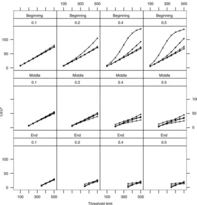
Fig. 3. EstimatedCED∗

(τ )against the values of the thresholdA. The first row of plots corresponds to the homogeneous scenarios (Hom) while the second row corresponds to the inhomogeneous scenarios (Inh). The different columns correspond to different values ofε. Each plot has three lines. The circles correspond to caseB, when the cluster emerges soon in the observation period (τ =50). The crosses correspond to caseM(τ =150), and the triangles correspond to caseL(τ=300).

to

τ

, the usual definition ofCEDis the expected number of observations one needs to wait until the alarm signal. That is,

CED

(τ )

=

E

[

TA

−

τ

|

TA

≥

τ

]

. One problem with this definition in the space–time situation is that all events between

τ

and TAcontribute toCED, either they belong to the cluster or not. We think that a more appropriateCEDdefinition is the average

number of events within the space–time cluster until the alarm goes off. We denote this measure byCED∗_{to distinguish it}

from the more usual temporal definition.

We tested with four different values for the spatial radius

ρ

: 0

.

25

,

0

.

5

,

1, and 2. It is worth remembering that the cluster basis is an unit square. We considered a more refined grid for values of the thresholdAthan in the without cluster scenario. Namely, we setAequal to 50

,

100

,

150

,

200

,

250

,

300

,

350

,

400

,

450, and 500.

The plots inFig. 3show the estimatedCED∗

_{(τ )}

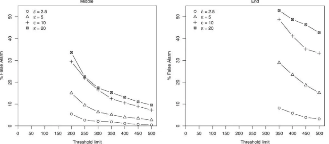
_{against the values of the thresholdA. The first row of plots corresponds to}

Fig. 4. Left hand side: False alarm rates versus threshold limitAfor the scenarios when the cluster emerges on the middle of the observation period with ε=2.5,5,10,20. Right hand side: Idem for cluster emerging at the end of the observation period.

We analyze initially only the the Middle and End scenarios. In these cases, the plots inFig. 3lead to the preliminary conclusion that the larger the

ε

, the better the performance of the surveillance method. Indeed, theCED∗

_{(τ )}

_{decreases with}

the increase of

ε

. One should rather set

ε

=

0

.

5 than

ε

=

0

.

2, which is the true value used in the simulation.

However, increasing

ε

too much leads to very large false alarm rates.Fig. 4shows the false alarm rates for

ε

equal to 2

.

5

,

5

.

0

,

10, and 20 in the homogeneous scenarios. The left hand size plot corresponds to the Middle and the right hand side to the End scenario. Then, it is clear that increasing

ε

without bounds renders the method useless because the false alarm rate is beyond tolerable standards. This behavior is virtually identical in the inhomogeneous scenarios.

Returning to the more practically oriented values of

ε

shown inFig. 3, we see that the delay for the alarm to go off is smaller if the cluster is at the end of the observation period. Basically, this means that the alarm system learns what is the intensity for a long time under the no cluster situation. When a cluster finally starts emerging, it is quickly detected. Unless the cluster is at the beginning of the observation period, theCED∗

(τ )

curves are almost parallel lines. Hence, the effect of the emerging time

τ

in theCED∗

(τ )

is approximately linear, unless

τ

is close to zero.

There is a heavy penalty for clusters located at the beginning of the observation period and with

ε

larger than the true relative change in intensity. In this situation, the expected delay increases very quickly. The alarm system takes a very long time to tell apart what is the baseline intensity from the emerging cluster higher intensity.

Contrasting the homogeneous with the inhomogeneous case, we can see fromFig. 3that, in the inhomogeneous case, the

CED∗

(τ )

is greater than in the homogeneous case. This effect is especially dramatic if the cluster is located in the beginning of the observation period and

ε

is larger than the true relative change.

InFig. 5, we show the effects of the radius

ρ

on the surveillance system performance for the homogeneous case. We ran simulations of the homogeneous scenario with spatial radius

ρ

=

0

.

25

,

0

.

5

,

1, and 2. The inhomogeneous case has virtually identical conclusions and it is not shown. The relative change parameter

ε

had the values 0

.

1

,

0

.

2

,

0

.

4, and 0

.

5. With respect to the observation period, the clusters started early (

τ

=

50), at the middle (

τ

=

150), or late (

τ

=

300). Most often, the procedure is insensitive to the choice of the radius

ρ

. Except for the cluster at the beginning and large

ε

, there is very little difference on the estimatedCED∗

_{(τ )}

_{. The exceptional behavior occurs only in a special conjunction of factors: when the}

parameter

ρ

is larger than the true cluster radius, when the clusters starts emerging early, and when

ε

is much larger than its true value.

6. Illustrative examples

We illustrate our method using two real datasets: the Burkitt’s lymphoma cases in Uganda, the same dataset used in

Rogerson(2001), and theMeningitiscases occurred in Belo Horizonte, Brazil, between 2001 and 2005.

6.1. Burkitt’s lymphoma cases in Uganda

A classical example of retrospective detection of space–time clustering is that based on the Burkitt’s lymphoma in Uganda (Williams et al., 1978). The data consist of the place of residence and onset time for all 188 cases of Burkitt’s lymphoma between 1961 and 1975 in the West Nile district in Uganda (seeFig. 6).Rogerson(2001) found evidence of space–time clusters using local Knox tests and adopting a probability of false alarm of 0

.

1. Notwithstanding the problems found in Rogerson’s method byMarshall et al.(2007), we compare our results with his.

Fig. 5. Effect of changingρ. The rows correspond to the three cluster emerging timeτ =50,150,300, and the columns correspond to different values ofε. Only the homogeneous case was considered. The curves with circles correspond toρ=0.25, the curves with triangle toρ=0.5, the curves with crosses toρ=1.0, and the curves with axes toρ=2.0. The true value ofρis 0.5.

number of observations. With respect to the emerging time

τ

, the estimates varied from 103 to 138. The largest number corresponds to the smallest radius (2.5). Except for this rather extreme radius, all the estimated starting times

τ

varied from 103 to 107, a very short range. More relevant than this, the estimated clusters are located approximately in the same region in all cases. Hence, the results are relatively insensitive to the tuning parameters values.

Fig. 6shows the graphs ofRnversusnfor

ρ

equal to 10 and 20 km. For

ρ

=

20 km and

ε

=

0

.

5, the alarm goes off

at event number 148 (February, 1973) and the method estimates that the clusters started on event 107 (November, 1970). This cluster is represented in the map on the right hand ofFig. 6. Note that, among the 40 events occurring all over the map between November, 1970 and February, 1973, only 20 belong to the cluster.

It is notable that the cases in the emerging cluster shown inFig. 6coincide with one of the clusters identified byWilliams et al.(1978) through the pairs of cases whose disease onset was in the period 1972–1973, within 10 km apart and 180 days of each other.

Rogerson(2001) ran his procedure with several different tuning parameters and his results are sensitive to these choices. Many of his detected clusters coincide with ours. However, one should keep in mind the criticisms to Rogerson procedure presented inMarshall et al.(2007).

We ran the space–time prospective scan statistic method proposed byKulldorff(2001) and implemented in the software SaTScan (Kulldorff, 2006). SaTScan is a freely available software and it was developed under the joint auspices of Martin Kull-dorff, the National Cancer Institute, and Farzad Mostashari of the New York City Department of Health and Mental Hygiene. There are difficulties comparing our method with that ofKulldorff(2001). His method, as implemented in the software, receives a dataset and scans for an alive cluster. That is, it searches for a cylinder-shaped cluster whose height ends at the last available observation time. Running his method with all 188 events will not allow for clusters that could have been found before the last observation. To avoid running his method manually repeatedly by adding a single observation each time, we ran it initially with all 188 observations. The scan statistic finds a non-significant cluster centered at the spatial coordinates (273, 332), with a radius equal to 13.42 km, and ranging from 9

/

2/1972 to 10

/

24/1975, when the scan alarm sounded off. Based on 999 simulations, the Monte Carlo p-value associated with this space–time cluster is equal to 0.129.

We then used this same 13.42 km radius found by the scan statistic in our own method. The alarm sounded off four times, in 6

/

15/1973, 4

/

24/1973, and 2

/

1/1973, for

ε

equal to 0.1, 0.2, 0.4, and 0.5, respectively. The clusters found were all centered at the spatial coordinates

(

273

,

332

)

, the same non-significant cluster found by the scan statistic based on all data points. Our method estimated the cluster emergence at 31

/

3/1971.

Fig. 6. Burkitt’s lymphoma cases in West Nile district of Uganda from 1961 to 1975 (study region is approximately 80 km×170 km). The left hand side map shows all the events in the period while the right hand side map shows the events identified in the emerging cluster by our method. Each one of the plots showsRnversusnfor four different choices ofε: 0.1,0.2,0.4, and 0.5. The left hand side plot usesρ =10 km and the right hand side plot uses ρ=20 km.

as our own method. A 5% significant cluster is found with radius equal to 11.40 km centered at

(

273

,

332

)

, and ranging from 2

/

9/1972 until the corresponding endpoint. Running Kulldorff’s procedure with the events until 2

/

1/1973, we find a 5% significant cluster with radius equal to 5.0 km centered at the spatial coordinates

(

263

,

333

)

, and emerging at 9

/

2/1972, the same date as the previous cases. Therefore, in this example, the two methods give similar results.

6.2. Meningitis cases in Belo Horizonte

We apply our method using data with place and onset date for 1001 Meningitis cases that occurred between 2001 and 2005 in Belo Horizonte, Brazil (seeFig. 7). In 60% of the days no cases were recorded and, in 72% of the remaining days, only one case was recorded. The maximum number of cases in a single day was equal to 6. From the time series plots inFig. 7, no discernible trend or periodicity is present.

The tested the following parameters:

ε

=

0

.

1

,

0

.

2

,

0

.

4, and 0

.

5;

ρ

=

1

,

2

,

3, and 4 km; alarm thresholdA

=

500. ThresholdA

=

500 means that we expect 500 cases before the alarm goes off without need. Since we have around 200 cases per year, we are expecting two unmotivated alarms in a period of 5 years.

Fig. 7. Map of Belo Horizonte divided into neighborhoods and the location of 1001 Meningitis cases that occurred between 2001 and 2005. The study region has approximately 31 km×16 km. The time series plots show the number of events in different time units: fortnightly, monthly, and quarterly. Each one of the plots showsRnversusnfor four different choices ofε: 0.1, 0.2, 0.4, and 0.5. The threshold isA=500. The left hand side plot usesρ=1 km and the right hand side plot usesρ=2 km.

Fig. 7shows theRnstatistics(2)versusnfor

ε

=

0

.

1

,

0

.

2

,

0

.

4

,

0

.

5 and

ρ

=

1

.

0

,

2

.

0 km. These plots illustrate the effects

of changing

ρ

and

ε

.

City health officials were not suspicious of any emerging cluster during this period before our analysis. Since the triggering event occur around the expected time under the no cluster situation, our method supports this opinion. There is no convincing evidence for the emergence of meningitis clusters in Belo Horizonte.

This lack of evidence is reinforced by Kulldorff’s prospective scan statistic method. Running his method with all the events, we did not find a significant cluster. Its most likely cluster, with p-value equal to 0.129, had radius zero, including only two events with identical spatial coordinates.

7. Conclusions

We avoid this problem by adopting the quality control ideas of average run length but our method requires the specification of tuning parameters. Although we think that users should be able to propose reasonable values for these parameters, one needs more studies to understand fully the impact of them in practice. This need to set tuning parameters is also a requirement inRogerson(2001) but, asMarshall et al.(2007) shows, his method has several shortcomings.

Our surveillance method assumes a spatially circular shaped cluster. A completely arbitrary shaped cluster is unfeasible computationally and circular shaped clusters provide a good trade-off between computational cost and meaningful and practical solutions. However, there are situations when a truly irregularly shaped cluster could be of concern such as a narrow zone along a river or an avenue. To solve this problem in the purely spatial cluster detection context, several authors have proposed spatial scan statistics using an irregular shaped scanning window (Duczmal and Assunção, 2004;Patil and Taillie, 2003;Duczmal et al.,2006;Tango and Takahashi, 2005;Assunção et al.,2006). Such scanning windows could also be adopted for our space–time statistic with some cost in additional computing time.

Our method has many desirable features. First, it does not require information about the population at risk, only cases are necessary. Second, it adjusts for purely spatial and purely temporal clustering, and it provides statistical inference for the emerging cluster detected. Third, it does not require many input parameters and the ones it does have a clear practical interpretation. This interpretation should help the user to establish reasonable values for them. We think it will be of great use in many practical applications.

Our method has been implemented in a stand-alone C++ software as well as in TERRAVIEW, a free GIS software based on the open-source TERRALIB library (seehttp://www.dpi.inpe.br/terraview/index.php). A suite of R functions has also been developed and they are available upon request.

References

Assunção, R., Costa, M., Tavares, A., Ferreira, S., 2006. Fast detection of arbitrarily shaped disease clusters. Statistics in Medicine 25, 723–742. Assunção, R., Maia, A., 2007. A note on testing separability in spatial-temporal marked point processes. Biometrics 63, 290–294.

Assunção, R., Tavares, A., Correa, T., Kulldorff, M., 2007. Space–time cluster identification in point processes. The Canadian Journal of Statistics 35, 9–25. Buckeridge, D.L., Burkom, H., Campbell, M., Hogane, W.R., Moore, A.W., 2005. Algorithms for rapid outbreak detection: A research synthesis. Journal of

Biomedical Informatics 38, 99–113.

Buehler, J.W., Hopkins, R.S., Overhage, J.M., Sosin, D.M., Tong, V., CDC Working Group, 2004. Framework for evaluating public health surveillance systems for early detection of outbreaks: Recommendations from the CDC Working Group. Morbidity and Mortality Weekly Report 7, 1–11.

Diggle, P.J., Rowlingson, B., Su, T.L., 2005. Point process methodology for on-line spatio-temporal disease surveillance. Environmetrics 16, 423–434. Duczmal, L.H., Assunção, R.M., 2004. A simulated annealing strategy for the detection of arbitrary shaped spatial clusters. Computational Statistics and Data

Analysis 45, 269–286.

Duczmal, L.H., Kulldorff, M., Huang, L., 2006. Evaluation of the spatial scan statistics for irregular shaped clusters. Journal of Computational and Graphical Statistics 15, 428–442.

Frisén, M., 2003. Statistical surveillance. Optimality and methods. International Statistical Review 71, 403–434.

Hardy, A., 2001. Methods of outbreak investigation in the ‘‘Era of Bacteriology’’ 1880–1920. Social and Preventive Medicine 46, 355–360. Henderson, D.A., 1999. The looming threat of bioterrorism. Science 283, 1279–82.

Höhle, M., 2007. Surveillance: An R package for the monitoring of infectious diseases. Computational Statistics 22, 571–582.

Höhle, M., Paul, M., 2008. Count data regression charts for the monitoring of surveillance time series. Computational Statistics and Data Analysis 52, 4357–4368.

Kenett, R.S., Pollak, M., 1996. Data-analytic aspects of the Shiryayev–Roberts control chart: Surveillance of a non-homogeneos Poisson process. Journal of Applied Statistics 23, 125–137.

Kulldorff, M., 2001. Prospective time periodic geographical disease surveillance using a scan statistic. Journal of the Royal Statistical Society, Series A 164, 61–72.

Kulldorff, M., 2006. SaTScanTM v7.0: Software for the Spatial and Space–time Scan statistics. Information Management Services, Inc., Available at

http://www.satscan.org/.

Kulldorff, M., Heffernan, R., Hartman, J., Assunção, R.M., Mostashari, F., 2005. A space time permutation scan statistic for disease outbreak detection. PLoS Medicine 2, 216–224.

Lawson, A.B., Kleinman, K., 2005. Spatial and Syndromic Surveillance for Public Health. Wiley, New York.

Marshall, J.B., Spitzner, D.J., Woodall, W.H., 2007. Use of the local Knox statistic for the prospective monitoring of disease occurrences in space and time. Statistics in Medicine 26, 1576–1593.

Mevorach, Y., Pollak, M., 1991. A small sample size comparison of the Cusum and the Shiryayev-Roberts approaches to change point detection. American Journal of Mathematical and Management Sciences 11, 277–298.

Patil, G.P., Taillie, C., 2003. Geographic and network surveillance via scan statistics for critical area detection. Statistical Science 18, 457–465. Pollak, M., 1985. Optimal detection of a change in distribution. Annals of Statistics 13, 206–227.

Pollak, M., Siegmund, D., 1985. A diffusion process and its application to detecting a change in the drift of Brownian motion. Biometrika 72, 267–280. Roberts, S.W., 1966. A comparison of some control chart procedures. Technometrics 8, 411–430.

Rodeiro, C.L.V., Lawson, A.B., 2006. Monitoring changes in spatio-temporal maps of disease. Biometrical Journal 48, 463–480.

Rogerson, P.A., 2001. Monitoring point patterns for the development of space–time clusters. Journal of the Royal Statistical Society, Series A 164, 87–96. Shiryaev, A.N., 1963. On the detection of disorder in a manufacturing process. Theory of Probability and its Applications 8, 247–265.

Sonesson, C., Bock, D., 2003. A review and discussion of prospective statistical surveillance in public health. Journal of the Royal Statistical Society, Series A 166, 5–21.

Tango, T., Takahashi, K., 2005. A flexibly shaped spatial scan statistic for detecting clusters. International Journal of Health Geography 4,

www.ij-healthgeographics.com/content/4/1/11 [05 October 2005].

Waller, L.A., Gotway, C.A., 2004. Applied Spatial Statistics for Public Health Data. John Wiley & Sons, New York.

Williams, E.H., Smith, P.G., Day, N.E., Geser, A., Ellice, J., Tukei, P., 1978. Space–time clustering of Burkitt’s lymphoma in the West Nile district of Uganda: 1961–1975. British Journal of Cancer 37, 109–22.