MODELLING OF BINARY MIXTURE COMMINUTION
F. E. P. SUDÁRIO and J. A. M. LUZ
Mining Eng. Department, Universidade Federal de Ouro Preto, Minas Gerais, Brazil. [email protected]
Abstract−− This paper treats on grindability dif-ferences of mineral mixtures to achieve a prelimi-nary selective particle size contrast by comminution in order to improve further sorting operation. Quartz and calcite had been chosen as example of binary system. The theoretical basis for this work was inspired by the optimization study carried out by Ray and Szekely (1973), through an algebraic model based on evolution of log-normal distribution of particle size during comminution. On the other hand, the present work has described grindability differences through the classical Rosin-Rammler size distribution. The study of the evaluation of binary mixture differences was realized by sieving analyses and the estimation of Rosin-Rammler sharpness and median diameter. An objective function was con-ceived stressing the relationship between the ex-pended energy in the grinding process and the opti-mum residence time. It is possible to use the results as a background for grinding optimization system, since that the penalty function inside objective func-tion can be adequately calibrated as far as technical and economic impacts on further sorting separations are concerned.
Keywords−− grindability; granular media; Rosin-Rammler; unit operations.
I. INTRODUCTION
Currently, it is well known that the selection and break process of the particle in the comminution is obtained by impact breaking, compression and abrasion. Know-ledge of the forces acting on particles in the different types of ores can contribute for the improvement of mineral processing. Several models were created to de-scribe forces acting on the particles during the break process. The formalism that has been by far most used is the population balance (King, 2001; Beraldo, 1987).
The critical operation in the processing of minerals is sorting. For their achievement, it is usual to apply comminution to achieve the necessary liberation. Ores constituted of minerals displaying differences in hard-ness, cleavage, parting and grindability have possibili-ties of economic gain in a processing plant, by particle size differentiation of the species to be separated. Such an optimum size contrast between the two species meets the compromise among the following parameters: libe-ration degree, selective size difference of components, concentration efficiency and specific energy consump-tion.
Modeling of comminution usually is performed em-ploying the population balance approach. This method
is based in two stochastic functions: the selection func-tion (linked to probability of each particle being selected in a single comminution event) and the breakage func-tion, which quantifies the progeny’s size distribution (Fuerstenau et al., 2003; Beraldo, 1987). So the model can predict particle size distribution of product after comminution. Non linearities in model equations can jeopardize the accuracy of the simulation, as already pointed out by Aboukheshem et al. (1986) and Bilgili and Scarlett (2005). Alternatively, using Lagrange’s multipliers method, Otwinowski (2006) has applied the maximum informational entropy to determine the brea-kage function.
Another interesting approach was used by Ray and Szekely (1973), who used a objective function based on maximization of the benefit that a selective comminu-tion gives to the subsequent process with a penalty cost function for comminution. They used the difference be-tween the mean sizes at the exit of the mill as quantifi-cation criterion for the benefit. These authors used the
discrete maximum principle for optimization in
sys-tems of decomposed structure. The model is based in the population balance model obeying the log-normal distribution, which is described by:
( )
(
)
2
2
log log 1
exp
2 log
log 2
d d
y d
σ
σ π
⎧ ⎡ − ⎤⎫
⎪ ⎢ ⎥⎪
= ⎨−⎢ ⎥⎬
⎪ ⎣ ⎦⎪
⎩ ⎭
(1)
where d is the median diameter of the particle; σ2 is the variance of size distribution of the material; y(d) is the fraction of material with diameters between d and d + Δd. Modifying such an approach of mixture commi-nution modeling the present work has studied the beha-vior of an binary ore in the grinding process, using a synthetic quartz and calcite mixture. The theoretical re-sults obtained by Ray and Szekely through the interac-tion of two materials of different grindability (said A and B) were found by using the log normal size distribu-tion and linking the intersecdistribu-tion area of the curves for material A and B with the possible separation capability of post-comminution equipment, associated to differ-ences of mean sizes and standard deviations as discri-minant parameters.
In parallel to this work Rosa and Luz (2010a; 2010b) had studied selective grinding of binary mixtures, aim-ing to simulate it by artificial neural network.
II. METHODS
as control. Isolated calcite and quartz were studied and also binary mixture with 20 %, 40 %, 60 %, and 80 % of calcite. Milling times were: 300 s, 900 s, 1800 s, 3600 s and 7200 s.
Firstly, all quartz and the calcite samples was pre-viously crushed (separately) below 3.35 mm. Repre-sentative sample mass for grinding tests was calculated according to Gy’s method (Wills and Napier-Munn, 2005).
Ball diameter was selected with aid of the Bond eq-uation (Beraldo, 1987). The steel mill used was unlined and had the following dimensions: 200 mm diameter and 200 mm in length. The tests were conducted in batch and dry operation.
The mainly used software for curve fitting and sta-tistical analysis was EasyPlot for Windows, version 4.0.4. Its algorithm uses a Marquardt-Levenberg filter, which, opposed the simplex search algorithm, allows the estimation of uncertainties associated with the val-ues of regression (Luz, 2005). Fitting curves of the me-dian diameter and the sharpness versus grinding time was obtained using FindGraph (software by UniPhiz Lab). Math derivation was done using the program Ma-thematica 7, that is a computer program for program-ming, mathematical modeling, simulation, data manipu-lation, graphical visualization, supporting several re-search areas, developed by Stephen Wolfram, Wol-fram’s. Algorithms were developed in Scilab.
Sieving tests were performed in duplicate for all samples. The experimental size data were input for sta-tistical fitting of Rosin-Rammler curves using Easyplot. After the fitting process, sharpnessand median diameter were used for simulating purposes. Behavioral analysis of calcite and quartz was carried out through the evolu-tion of median diameter and the sharpness of the Rosin-Rammler distribution:
( )
501 exp ln 0,5
m
i i
d Y
d
⎡ ⎛ ⎞ ⎤
⎢ ⎥
= − ⎜ ⎟
⎢ ⎝ ⎠ ⎥
⎣ ⎦
(2) where: Yi is the fraction of the material passing through
size class i[-]; di is the size (diameter) of class i [m]; d50
is the median diameter of particle size distribution [m]; m is the sharpness parameter [-]. The higher the sharp-ness, the narrower the range of the distribution is.
0 2000 4000 6000 8000 10000 12000
5 15 25 35 45 55 65 75
Two‐Teta [deg]
Int
e
ns
it
y
[c
o
unt
s]
0 2000 4000 6000 8000 10000 12000 Calcite Sample Quartz Sample
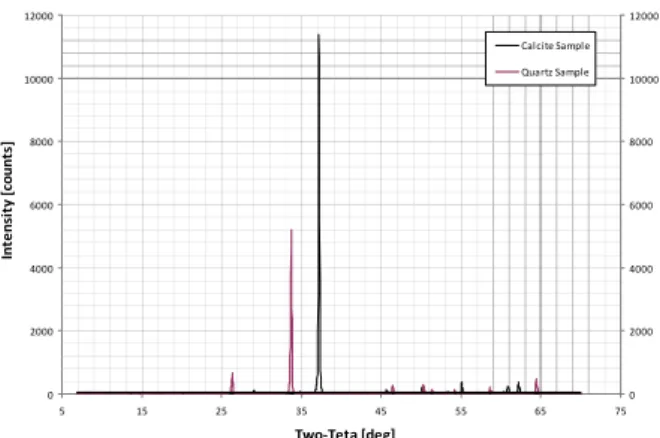
Fig. 1: Diffractograms of quartz and calcite.
Calcite content in the mixture in each size class was es-timated by loss of ignition at 950 ºC (for 3,600 seconds). The weight loss corresponded to the evolution of CO2, permits the stoichiometric calculation of the calcite content in the mixture.
X-ray diffraction analysis has confirmed the micro-structure of quartz and calcite crystals. The two diffrac-tograms met respectively the standard patterns for cal-cite and quartz (Fig. 1).
III. RESULTS AND DISCUSSION
The interesting aspect in this work is the mutual influ-ence of the proportion of quartz and calcite in the binary mixture, measured by the differences in size distribu-tion, since the sharpness evolution of the mixture with grinding time showed the influence that a mineral does workout over the other one, as comparing with results obtained by grinding each one separately.
This work was completed with an objective function obtained through empirical and theoretical results which relates the intersection area of the curves of quartz and calcite with a penalty function depending on the (cost related) time of grinding.
The results of particle size analysis of each isolated material by Rosin-Rammler curve fitting are shown in Fig. 2 and 3 (whose experimental conditions are sum-marized in Tables 1, 2, 3 and 4).
The operational conditions and the symbols for curves of Fig. 2 are systematized in Table 1 and the conditions referring the Fig. 3 shown in Table 2.
The mutual influence of mineralogical species of the binary mixtures (calcite and quartz in proportion 60%:40% ; 40%:60%; 20%:80 %; and 80%:20 %) was studied and can be inferred from analysis of Figs. 4 to 7. The operating conditions and the symbols used for the curves of Fig. 4 are systematized in Table 3.
0 10 20 30 40 50 60 70 80 90 100
10 100 1000 10000
C
u
m
u
lat
ive
p
assi
n
g
[
%
]
Size [µm]
Fig. 2: Evolution of particle size distribution of isolated quartz with Rosin-Rammler regression.
Table 1: Distribution size evolution of quartz and the Rosin-Rammler curve (data of Fig. 2)
Grinding
time [s] Sharpness
Median diame-ter [µm] R
2 Symbol in
Figure 2 0 1.40 1568 0.999
300 1.40 1084 0.999 c 900 1.35 658 0.998 z 1800 1.33 463 0.997
3600 1.31 319 0.996 {
0 10 20 30 40 50 60 70 80 90 100
10 100 1000 10000
C
u
m
u
la
ti
v
e
p
a
s
s
in
g
[
%
]
Size [µm]
Fig. 3: Evolution of particle size distribution of isolated cal-cite with Rosin-Rammler regression.
Table 2: Distribution size evolution of calcite and the Rosin-Rammler curve (data of Figure 3).
Grinding
time [s] Sharpness
Median diame-ter [µm] R
2 Symbol in
Figure 3 0 1.01 1754 0.998
300 1.13 830 0.998 c 900 1.10 458 0.998 z
1800 1.26 312 0.997
3600 2.00 223 0.999 {
7200 2.85 162 1.000 U
0 10 20 30 40 50 60 70 80 90 100
10 100 1000 10000
C
u
m
u
lat
ive
p
assi
n
g
[
%
]
Size [µm]
Fig. 4: Temporal evolution in the mixture of calcite (60 %) and quartz (40 %) with Rosin-Rammler regression.
Table 3: Distribution evolution of calcite (60 %) and quartz (40 %), and the Rosin-Rammler curve (data of Figure 4).
Grinding
time [s] Sharpness
Median diame-ter [µm] R
2 Symbol in
Figure 4 0 1.14 1659 0.998
300 1.24 858 0.999 c
900 1.37 565 0.999 z
1800 1.49 440 0.995
3600 1.57 310 0.997 {
7200 1.64 174 0.994 U
0 10 20 30 40 50 60 70 80 90 100
10 100 1000 10000
C
u
m
u
la
ti
ve p
assi
n
g
[
%
]
Size [µm]
Fig. 5: Evolution of the global grain mixture of 40 % calcite and 60 % quartz with Rosin-Rammler regression (conditions and symbols are in Table 4).
Table 4: Distribution evolution of calcite (40 %) and quartz (60 %), and the Rosin-Rammler curve (data in Figure 5).
Grinding
time [s] Sharpness
Median diame-ter [µm] R
2 Symbol in
Figure 5 0 1.21 1721 0.998 300 1.32 1033 0.999 c 900 1.35 679 0.999 z 1800 1.45 468 0.998
3600 1.49 364 0.997 {
7200 1.45 215 0.996 U
0 10 20 30 40 50 60 70 80 90 100
10,0 100,0 1000,0 10000,0
C
u
m
u
la
ti
ve p
assi
n
g
[%
]
size [µm]
Fig. 6: Evolution of the global grain mixture of 80 % calcite and 20 % quartz with Rosin-Rammler regression (conditions and symbols are in Table 5).
Table 5: Distribution evolution of calcite (80 %) and quartz (20 %), and the Rosin-Rammler curve (in Figure 6).
Grinding
time [s] Sharpness
Median diame-ter [µm] R
2 Symbol in
Figure 6 0 1.08 1705 0.998
300 1.14 896 0.998 c
900 1.27 549 0.997 z
1800 1.37 379 0.997
3600 1.99 260 0.999 {
7200 1.66 179 0.995 U
0 10 20 30 40 50 60 70 80 90 100
10 100 1000 10000
C
u
m
u
la
ti
v
e
p
assi
n
g
[%
]
size [µm]
Fig. 7: Evolution of the global grain mixture of 20 % calcite and 80 % quartz with Rosin-Rammler regression (conditions and symbols are in Table 6).
Table 6: Distribution evolution of calcite (20 %) and quartz (80 %), and the Rosin-Rammler curve (data in Figure 7).
Grinding
time [s] Sharpness
Median diame-ter [µm] R
2 Symbol in
Figure 7 0 1.32 1596 0.999
300 1.36 1093 0.997 c 900 1.32 619 0.998 z
1800 1.25 418 0.998
3600 1.44 323 0.997 {
0 200 400 600 800 1000 1200 1400 1600 1800 2000
0 1000 2000 3000 4000 5000 6000 7000 8000
M
e
d
ian
d
iam
eter
[µ
m
]
Time [s]
100% quartz
100% calcite
40% calcite / 60% quartz
60% calcite / 40% quartz
Fig. 8: Median diameter evolution of the mixture of 40 % and 60 % calcite and of the isolated quartz and isolated calcite.
0 200 400 600 800 1000 1200 1400 1600 1800 2000
0 1000 2000 3000 4000 5000 6000 7000 8000
M
e
d
ian
D
iam
et
er
[µ
m
]
Time [s]
100% quartz
100% calcite
20% calcite / 80% quartz
80% calcite / 20% quartz
Fig. 9; Median diameter evolution of the mixture of 20 % and 80 % calcite and of the pure quartz and isolated calcite.
1,0 1,2 1,4 1,6 1,8 2,0 2,2 2,4 2,6 2,8
0 1000 2000 3000 4000 5000 6000 7000 8000 Time [s]
S
h
ar
p
n
e
ss [
-]
40%:60%
60%:40%
100% quartz
100% calcite
Fig. 10: Sharpness evolution for mixtures of 40 % and 60 % calcite and of the isolated quartz and isolated calcite.
1,0 1,2 1,4 1,6 1,8 2,0 2,2 2,4 2,6 2,8
0 1000 2000 3000 4000 5000 6000 7000 8000 Time [s]
S
h
ar
p
n
e
ss [
-]
20%:80%
80%:20%
100% quartz
100% calcite
Fig. 11: Sharpness evolution for mixtures of 20 % and 80 % calcite and of the isolated quartz and isolated calcite.
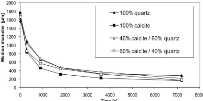
Aiming the detection improvement of the composi-tion effect on grindability of binary mixtures, the re-gression values corresponding to the average size (d50)
and the sharpness of the distribution of each mixture (m) were plotted in Figs. 8, 9, 10 and 11.
The evolution of median diameter, referring to the various mixtures studied is shown in graphs of Fig. 8 and 9. It is seen that there was typical behavior for the
median diameter for comminution processes, since there was systematical decrease of graining with the increas-ing millincreas-ing time. Note also, the typical behavior of asymptotic attenuation of the curve (fact well known in the industry).
According to the temporal evolution of sharpness in Rosin-Rammler distribution referred to the global mix, it can be seen in Fig. 10 and 3.11. It should be remem-bered that the parameter m (the sharpness) is a measure of dispersion (analogous to standard deviation), contrary to the median diameter, which is a measure of central tendency. It can be seen that isolated quartz and calcite behave differently. In the quartz there is a tendency to preserve the amplitude distribution with a slight de-crease in sharpness and increasing milling time.
Pure calcite (which exhibits perfect cleavage) shows a great increase in sharpness with the milling time, showing the effect of preferential breakage of larger particles in a population initially with broader size dis-tribution range.
In order to detect possible effects in the sharpness evolution of a mineral over the other one, it was also calculated a theoretical and hypothetical sharpness of the mixture, in case there were no mutual interference in the components of the mixture under comminution. This hypothetical sharpness was taken as the weighted aver-age of values for the isolated minerals, having as weight factor the proportion of phases (calcite and quartz).
Figures 10 and 11 show the influence of the quartz in calcite grindability, when compared to isolated cal-cite, with the same milling time.
The comparison between hypothetical and experi-mental values are seen in Fig. 12 and 13. Fig. 10 and 11 show the difference in size distribution between quartz,
1,0 1,2 1,4 1,6 1,8 2,0 2,2 2,4
0 1000 2000 3000 4000 5000 6000 7000 8000
S
ha
rpne
s
s
[
-]
Time [s]
weighted average of the sharpness: 40%:60% weighted average of the sharpness: 60%:40% 40%:60%
60%:40%
Fig. 12: Sharpness evolution of the simulated and real mixture for mixtures of 40 %:60 % calcite (solid squares).
1,0 1,2 1,4 1,6 1,8 2,0 2,2 2,4 2,6
0 1000 2000 3000 4000 5000 6000 7000 8000
S
h
ar
p
n
e
ss [
-]
Time [s] 80%:20%
20%:80%
weighted average of the sharpness: 80%:20% weighted average of the sharpness: 20%:80%
Table 7: Relative deviation of the sharpness of the mixture distribution.
Mixture of 40 % calcite and 60 % quartz
Mixture of 60 % calcite and 40 % quartz
Time [s] Experimental Weighted Relative
deviation [%] Experimental Weighted Relative deviation [%]
0 1.21 1.24 -2.81 1.14 1.17 -2.28 300 1.32 1.29 2.12 1.24 1.24 0.16 900 1.35 1.25 7.41 1.37 1.20 12.41 1800 1.45 1.30 10.21 1.49 1.29 13.56 3600 1.49 1.59 -6.44 1.57 1.72 -9.81 7200 1.45 2.05 -41.10 1.64 2.31 -41.10
Table 8: Relative deviation of the sharpness in mixture distri-bution.
Mixture of 20 % calcite and 80 % quartz
Mixture of 80 % calcite and 20 % quartz
Time [s] Experimental Weighted Relative
deviation [%] Experimental Weighted Relative deviation [%]
0 1.20 1.32 -9.47 1.09 1.09 0.18 300 1.36 1.35 1.03 1.14 1.18 -3.86 900 1.32 1.30 1.52 1.27 1.15 9.45 1800 1.25 1.32 -5.28 1.37 1.27 7.01 3600 1.44 1.45 -0.56 1.99 1.86 6.43 7200 1.63 1.78 -9.08 1.66 2.58 -55.54
0% 20% 40% 60% 80% 100% 120%
10 100 1000 10000
C
u
m
u
la
ti
ve p
assi
n
g
[
%
]
Opening [µm]
Fig. 14: Size distribution evolution of calcite in mixture cal-cite/quartz in proportion 40 % : 60 % (virtually isolated).
0% 20% 40% 60% 80% 100% 120%
C
u
m
u
lat
ive p
ass
in
g
[
%
]
Opening [µm]
Fig. 15: Size distribution evolution of calcite in mixture cal-cite/quartz in proportion 60 % : 40 % (virtually isolated).
calcite and mixtures using values of sharpness parame-ter. The independence or not between quartz and calcite can also be evaluated by analyzing the sharpness para-meter. Figures 12 and 13, show the curves that represent the condition for which the calcite and quartz behave independently during milling hypothetical, and the curves that represent the actual situation obtained by experiments.
Tables 7 and 8 show the relative deviations between empirical and hypothetical values (weighted average) of the sharpness in the mixtures. It can be seen clearly that there is interference, because the deviations are
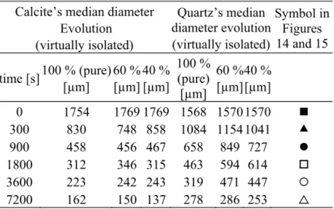
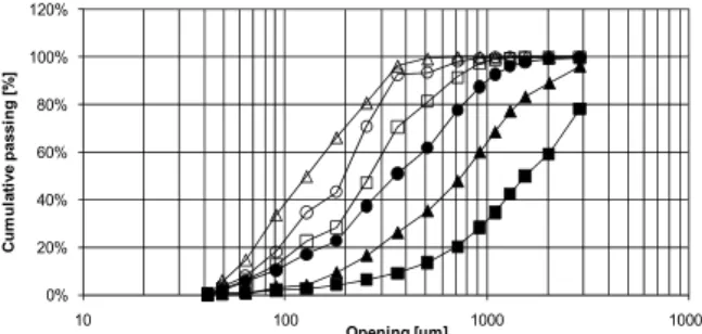
appreci-able for larger grinding times. The first point of tappreci-able 8 was aberrant, indicating experimental error. Anyway, as the relative deviations are appreciable, the hypothesis of no interference can be ruled out. The effects of mutual interference in the comminution of the two mineralogi-cal species in mixture are more representative plotting the evolution of the two minerals separately. This is equivalent to consider when studying a given compo-nent that the other one would be part of the grinding media. The values of calcite and quartz sizes (virtually isolated) in function of grinding time are shown in Figs. 14, 15, 16 and 17.
Operational conditions for curves of Figs. 14 and 15 are in Tables 9 and 10, and operational conditions for curves of Figs. 16 and 17 are in Tables 11 and 12.
A. Mathematical Model of the Size Distribution Con-trast.
Fitting was made according to the Rosin-Rammler curve (Eq. 3) in relation to the cumulative passing of all material. The form of the equation found for the median diameter in relation to the time from 0 to 7,200 seconds was:
exp t
y a c
b
⎛ ⎞ = × ⎜− ⎟+
⎝ ⎠ (3)
where, t is time (seconds); a, b e c are constant.
The sharpness in relation to the time from 0 to 7,200 seconds was fitted to:
3 2
y= × + × + × +a t b t c t d (4) where, t is time (seconds); a, b, c and d are constants.
Table 9: Composition effect on temporal evolution of median diameter.
Calcite’s median diameter Evolution (virtually isolated)
Quartz’s median diameter evolution (virtually isolated)
Symbol in Figures 14 and 15
time [s]100 % (pure) [µm]
60 % [µm]
40 % [µm]
100 % (pure) [µm]
60 % [µm]
40 % [µm]
0 1754 1769 1769 1568 1570 1570
300 830 748 858 1084 1154 1041 c 900 458 456 467 658 849 727 z
1800 312 346 315 463 594 614
3600 223 242 243 319 471 447 {
7200 162 150 137 278 286 253 U
Table 10: Composition and temporal evolution of sharpness, m. Calcite’s sharpness
evolution (virtually isolated)
Quartz’s sharpness evolution (virtually isolated)
Symbol in Figures 14 and 15 Time
[s] 40% 100 %
(pure) 60 % 40 % 100% (pure) 60 % 0 1.04 1.01 1.04 1.04 1.40 1.43
300 1.20 1.13 1.18 1.20 1.40 1.45 c
900 1.30 1.10 1.39 1.30 1.35 1.54 z
1800 1.60 1.26 1.71 1.60 1.33 1.64
3600 1.77 2.00 1.79 1.77 1.31 1.65 {
0% 20% 40% 60% 80% 100% 120%
10 100 1000 10000
C
u
m
u
la
ti
ve p
assi
n
g
[
%
]
Opening [µm]
Fig. 16: Size distribution evolution of calcite in mixture cal-cite/quartz in proportion 20 % : 80 %.
0% 20% 40% 60% 80% 100% 120%
10 100 1000 10000
C
u
m
u
la
tiv
e
p
a
s
s
in
g
[
%
]
Opening [µm]
Fig. 17: Size distribution evolution of calcite in mixture cal-cite/quartz in proportion 80 % : 20 %.
Table 11: Composition and evolution of diameter.
Calcite’s median diameter Evolution (virtually isolated)
Quartz’s median di-ameter evolution (virtually isolated)
Symbol in Figures 16 and 17
tempo [s] 100 % (pure) [µm]
20 % [µm]
80 % [µm]
100 % (pure) [µm]
20 % [µm]
80 % [µm]
0 1754 1769 1769 1568 1570 1570 300 830 747 826 1084 993 1106 c 900 458 377 499 568 768 766 z 1800 312 270 394 463 611 521
3600 223 186 252 319 521 411 {
7200 162 139 143 278 285 251 U
Table 12: Composition effect on evolution of sharpness, m.
Calcite’s sharpness Evolution (virtually isolated)
Quartz’s sharpness evolution (virtually isolated)
Symbol in Figures 16 and 17 tempo
[s]
100 %
(pure) 20 % 80 % 100 %
(pure) 20 % 80 % 0 1.01 1.04 1.04 1.40 1.43 1.43
300 1.13 1.29 1.21 1.40 1.33 1.37 c
900 1.10 1.26 1.38 1.35 1.36 1.47 z
1800 1.26 1.51 1.60 1.33 1.43 1.53
3600 2.00 1.85 1.88 1.31 1.79 1.61 {
7200 2.85 1.72 1.92 1.51 2.01 1.54 U
In order to quantify (in specific grinding time) the particle size contrast between the components, it is con-venient to express this contrast in terms of intersection area between the two size distribution curves (Fig. 18).
The intersection (I) between the fitted Rosin-Rammler curves of calcite and quartz (Fig. 18) can be
obtained by analytical procedure. The values of sharpness and the median diameter in relation to the time were found by the fitting curve shown in the Eqs. 3 and 4.
Such equations were incorporated into the Rosin-Rammler probability density equation:
1
0 0 0
exp
m m
m x x
f
x x x
− ⎡ ⎤
⎛ ⎞ ⎛ ⎞
⎢ ⎥
= ×⎜ ⎟ × −⎜ ⎟
⎢ ⎥
⎝ ⎠ ⎣ ⎝ ⎠ ⎦
(5) The scale parameter (x0) is obtained by the relationship:
50
0 1
1 ln
2
m
x x =
⎡ ⎛ ⎞⎤ − ⎜ ⎟ ⎢ ⎝ ⎠⎥
⎣ ⎦
(6)
Considering the curve fA in the Figure 3.17 as being
calcite and fB as the quartz curve, in the intersection one
has:
(
,)
(
,)
0A I I B I I
f x y − f x y = (7)
The roots of this equation provide, naturally the in-tersection points of curves of the two components in the mixture in comminution, which are the coordinates xI
and yI. Equation 7 can be expressed by:
1
0 0 0
1
0 0 0
exp
exp 0
A A
B B
m m
A I I
A A A
m m
B I I
B B B
m x x
y
x x x
m x x
x x x
−
−
⎡ ⎤
⎛ ⎞ ⎢ ⎛ ⎞ ⎥
= ×⎜ ⎟ × −⎜ ⎟ −
⎢ ⎥
⎝ ⎠ ⎣ ⎝ ⎠ ⎦
⎡ ⎤
⎛ ⎞ ⎢ ⎛ ⎞ ⎥
×⎜ ⎟ × −⎜ ⎟ =
⎢ ⎥
⎝ ⎠ ⎣ ⎝ ⎠ ⎦
(8)
To implement the mathematical model, it was made the Newton-Raphson algorithm in Scilab for time from 0 to 7,200 seconds, with span of 10 seconds. Through this algorithm it was found the intersection values between the Rosin Rammler probability density equation of quartz and calcite. As Newton-Raphson method requires deriva-tion of eq. 8, this was done using the program Mathema-tica 7, generating the following expression:
1 2 3 4
'( ) '( ) '( ) '( ) '( ) f x = f x + f x + f x + f x
(9) Being:
Newton-Raphson algorithm to find intersection val-ues between the Rosin-Rammler density equation of quartz and calcite was made in Scilab, for 0 s to 7,200 s (time span of 10 seconds). After finding the value I = (xI;yI), the calculation of the areas A1 and A2 can be
done using the Rosin-Rammler cumulative distribution (integral), resulting the equation:
(
)
2
0
Area A 1 1 exp
A
m I A i
A
x
Y x x
x
⎡ ⎛ ⎞ ⎤
⎢ ⎥
= − = = − ⎢−⎜ ⎟ ⎥
⎝ ⎠
⎣ ⎦ (10)
(
)
1
0
Area A exp
B
m I B i
B
x
Y x x
x
⎡ ⎛ ⎞ ⎤
⎢ ⎥
= = = − ⎜ ⎟
⎢ ⎝ ⎠ ⎥
⎣ ⎦
(11) The following expression is shown as an example of final expression for the areas calculation, and refers to the calculation of area A2 for the mixture with 20% cal-cite, in a generic time interval, t:
(
)
0
exp
m
I
A i
A x
Y x x
x
⎡ ⎛ ⎞ ⎤
⎢ ⎥
= = − ⎜ ⎟
⎢ ⎝ ⎠ ⎥
⎣ ⎦ (12)
being:
12 3 8 2 4
4,17 1,18 2,16 1,11
m= − e− t + e t− + e t− + (13)
50 1544 exp 216
300 t d = × ⎛⎜− ⎞⎟+
⎝ ⎠ (14)
1 50 0
1 ln
2
m A
d x =
⎡ ⎛ ⎞⎤ − ⎜ ⎟ ⎢ ⎝ ⎠⎥
⎣ ⎦
(15)
The objective function is then the sum of plot areas plus the cost weighted function, formed by multiplying a weight penalty function dependent (in a first ap-proach), only of the operation cost.
( )
( )
1 2
[( ) c ]
j ob
f =Minimize A+A + ×p f (16) where p is the weight factor and f(c) is the penalty func-tion, encompassing the cost which is especially depen-dent of the grinding time, since with increasing grinding time, results increased energy spending. Parameter p also depends on the economical benefit resulting on the subsequent sorting operations. In each concrete and ac-tual case this positive impact must be quantified usually by pilot scale testwork.
For grinding time, t, one has, after including the classical Bond’s comminution equation:
(
)
80 80
1 1
( ) , $ 10 t
f c f E q Q Wi
P F
⎛ ⎞
= = × × × ×⎜⎜ − ⎟⎟×
⎝ ⎠ (17)
where Q is the mass flowrate and q takes on account the other operational expenditures like grinding media and liners consumption, and so on (q>1).
The parameters: Wi, F80 and P80 of the previous
equ-ation are Bond’s work index, screen openings which pass 80 % of the feed and 80 % of the product respec-tively.
IV. CONCLUSIONS
With Rosin-Rammler equation one can detect difference between quartz and calcite with grinding time. The me-dian diameter evolves according to negative exponential law, and no sensible impact on the composition of the mixture in this parameter was seen, as the size distribu-tions of the two isolated minerals are concerned. The grinding progress did not affect significantly the sharp-ness parameter for quartz. The behavior of calcite, how-ever, shows that the progress of grinding leads to a in-crease in amplitude of particle size distribution.
The interdependence of the behavior of the two min-erals can be verified. The quartz presence during grind-ing of calcite led to increased sharpness parameter of calcite size distribution. This behavior is consistent with the fact that the calcite presents perfect rhombohedral cleavage, and lower hardness and strength as compared to quartz.
The results were promising to help decrease the cost of grinding and better sorting performance.
REFERENCES
Aboukheshem, M, K. Prisbrey, L.R. Bunnell and J.M. Lytle, “Fourier shape descriptors and particle brea-kage energy,” Particulate Science and Technology,
4, 143 – 149 (1986).
Beraldo, J.L., Moagem de Minérios em Moinhos Tubulares, Edgard Blücher, São Paulo (1987). Bilgili, E. and B. Scarlett, “Population balance
model-ing of non-linear effects in millmodel-ing processes,” Powder Technology, 153, 59–71 (2005).
Fuerstenau, D.W., P.C. Kapur and A. De, “Modeling Breakage Kinetics in Various Dry Comminution Systems,” KONA, 21, 121 -132 (2003).
King, R.P, Modeling & Simulation of Mineral Processing Systems, Butterworth-Heinnemann (2001).
Luz, J.A.M., “Conversibilidade entre distribuições probabilísticas usadas em modelos de hidrociclones,” Revista Escola de Minas, 58, 89-93 (2005).
Otwinowski, H., “Maximum entropy method in commi-nution modeling,” Granular Matter, 8, 239–249 (2006).
Rosa, G.M and J.A.M. Luz, “Seletividade na cominuição de mesclas de dolomita e quartzo,” Revista Escola de Minas, 63 (2010).
Rosa, G.M. and J.A.M. Luz, “Dry Grinding of Dolomite and Quartz and its Simulation by a Neural Net-work,” XIIth International Mineral Processing Sym-posium (2010).
Wills, B.A. and T. Napier-Munn, Mineral Processing Technology, B-H Elsevier, Amsterdam (2005).