AN LCMV-BASED APPROACH FOR DOWNLINK
BEAMFORMING IN FDD SYSTEMS IN PRESENCE OF
ANGULAR SPREAD∗
D. Zanatta Filho
1, C. C. Cavalcante
1, J. M. T. Romano
1and L. S. Resende
21
DSPCom
, FEEC, UNICAMP, Brazil
P.O. 6101, CEP: 13083-970, Campinas-SP, Brazil
{
daniloz,charles,romano
}
@decom.fee.unicamp.br
2
Federal University of Santa Catarina
P.O. 476, CEP: 88040-900, Florian´
opolis-SC Brazil
[email protected]
ABSTRACT
An approach based on constrained filtering for down-link beamforming for FDD systems is presented. The impact of the angular spread in the calculation of the beamforming weights is evaluated for such approach, as well as for that based on the maximization of the signal to interference ratio. It is shown that the LCMV-based method leads to an efficient solution with the introduc-tion of eigenvector constraints in the optimizaintroduc-tion pro-cedure. The simulation results illustrate the good per-formance of the proposed technique, which presents an acceptable computational complexity and is suitable for adaptive implementation.
1 INTRODUCTION
In mobile communications the downlink beamforming plays an important role in the increasing of link qual-ity and/or system capacqual-ity. Beamforming may be per-formed with or without cancellation of interferers. Fur-ther, the use of joint beamforming and cancellation pro-vides better results [1].
In this context, the main drawback concerns the downlink channel parameters (reverse link) which are not available prior to transmission and must be esti-mated in order to provide a correct beamforming. Such parameters can be the spatial covariance matrix or the DOAs (directions of arrival) together with the angular spread (AS) and the powers of each multipath. For TDD systems both parameters (spatial covariance matrix and DOA) are the same in up- and downlink, provided that time duplex distance is small enough, i.e., smaller than the coherence time of fading. However, for FDD systems where frequency duplex distance is greater than coher-ence bandwidth, an useful approach is to use uplink pa-rameters, obtained from received signal, to estimate the downlink ones [1, 2].
∗This work was supported by a grant from Ericsson of
Brazil Research Branch under ERBB-UNI.33 Technical Coopera-tion Contract.
After the up- to downlink mapping, the beamforming weights may be obtained from the estimated covariance matrix by means of the Summed Inverse Carrier to in-terference Ratio (SICR) criterion, as posed in [2, 3]. An alternative strategy is the Linearly Constrained Mini-mum Variance (LCMV) criterion. Such method con-sists on the minimization of the transmitted power with point constraints in the array response, so that the di-rections of the desired signals be enhanced [4, 5]. In the original method of LCMV the angular spread (AS) was not considered in order to find the weights for beam-forming. In this paper we investigate the inclusion of the AS on the LCMV-based solution by means of some additional considerations over the constraints to obtain satisfactory interference cancellation in presence of AS. The most suitable solution is the use of the so-called eigenvector constraints instead of the point one. AS can also be included in the previous method, based on the SCIR criterion. This allows us to evaluate the perfor-mance for both methods, providing comparative results. Such results indicate some performance equivalency be-tween both LCMV-based and SICR methods in presence of angular spread (AS).
The paper is organized as follows. Section 2 presents the LCMV solution with the introduction of eigenvec-tor constraints. Section 3 recalls the SICR criterion, so that the simulations and performance comparison for both methods are presented in Section 4. Finally, our conclusions are stated in Section 5.
2 LCMV-BASED SOLUTION
2.1 No Angular Spread
The LCMV is a criterion that minimizes both pollution1
and interference. In addition, the array response is con-strained to some values at defined directions in order to force the array to transmit for the desired user. This approach requires the knowledge of the DOA and the
power of each user multipath, in order to compute the corresponding constraints.
For each user, the beamforming weights are obtained by
wk = arg min
wk ©
wHkRwkª ¯¯CTkwk=fk (1)
where Ris the total (for all users) downlink covariance matrix, Ck is the constraint matrix for the k-th user
and fk is the response vector for thek-th user.
Such method just takes into account the correspond-ing DOAs for each user, by introduccorrespond-ing point constraints for each direction. That is, the signal (angular) spread around its DOA is not considered. The matrix Ck is
formed as follows:
Ck= £
d(θ1) d(θ2) · · · d(θL)
¤
(2) where d(θl) is the steering vector corresponding to the
l-th considered DOA andLis the number of constraints. The response vector is given by:
fk= £
1 √γ2 · · · √γL
¤T
(3) where γl is the relative power of thel-th path with
re-spect to the first one.
2.2 Angular Spread - Point Constraints
To deal with AS, a number of point constraints must be applied over the angle bandwidth. However, the number of antenna in the array limits the number of constraints, since each constraint requires two antennas and a certain degree of freedom is necessary to minimize the transmitted power in other directions. So, there are two possibilities: the use of the mean DOA or consider-ing a number of discrete DOAs in the angle bandwidth. Figure 1 depicts an example of 3 point constraints for a given AS.
DOA
AS/2 -AS/2
Figure 1: Point constraints for angular spread consider-ation.
A different strategy consists in avoiding point con-straints, as presented in the sequel.
2.3 AS - Eigenvector Constraints
As mentioned in the previous section, the use of point constraints is limited to the number of degree of free-dom. In order to increase the degree of freedom, the
so-called eigenvector (EV) constraints have been intro-duced by [6, 5].
EV constraints proceed from a lower rank orthonor-mal representation of the signal space, based on the Karhunen-Lo`eve discrete expansion [5]. Such represen-tation is obtained using the set of eigenvectors corre-sponding to the most significant eigenvalues of the de-sired user spatial covariance matrix. This is the most efficient representation of the signal space, in the statis-tical second order sense.
Furthermore, it can be also shown that EV constraints are based in a minimum square approximation of the desired array response over the desired user angle band-width. The EV constraints are optima in the sense that the mean square error between the obtained array re-sponse and the desired one is minimized for a given number of constraints [7]. Hence the EV constraints provide a more direct control over the array response than the point constraints.
In practice, the singular value decomposition (SVD) is directly applied to the point constraints matrix and a more simple representation ofCk is given as follows:
CHk =Uk ·
Σk 0
0 0
¸
VkH (4)
and
U=£ u1 u2 · · · uL
¤
V=£ v1 v2 · · · vM
¤
Σ= diag (σ1, σ2, . . . , σP)
(5)
where U and V are unitary matrices, containing the left and right singular vectors, respectively; and Σ is the diagonal matrix composed by the singular values of
Ck sorted asσ1≥σ2≥. . .≥σP >0.
For a given numberp≤P of constraints, the matrices
U,VandΣare reduced to:
e
U=£ u1 u2 · · · up
¤
e
V=£ v1 v2 · · · vp
¤
e
Σ= diag (σ1, σ2, . . . , σp)
(6)
Thus the EV constraints matrixCek and EV response
vectorefk are given by: e
CHk =VeH
efk =Σe−
1e
UHf k
(7)
The LCMVEVis then described by equations (6) and
(7) applied to (1).
3 SICR SOLUTION
proposed. The aim of this method is to maximize the transmitted power for the desired user and to cancel the others by placing spatial nulls in their direction. This criterion can be described as
γk = (CIR)k = max
w
1...wK
wkHRkwk K
P j=1
j6=k
wH j Rkwj
(8)
A sub-optimum solution for this problem can be found by means of a new criterion, defined as
arg max
w1...wK "K
X
k=1
γ−k1
#
(9)
With this new criterion, the sub-optimum beamform-ing weights can be independently performed as follows:
wk = arg max
wk
wH k Rkwk
wH
k Rk,intwk
(10)
where Rk and Rk,int = R−Rk = P i,i6=k
Ri+σ
2
nI are
respectively the downlink covariance matrix of the k-th user and k-th’s interferers plus noise, while wk is the
beamformer weight vector for thek-th user.
This minimization procedure can be solved by using Lagrange multipliers. The solution is the unit norm gen-eralized eigenvector of [Rk,Rk,int] corresponding to the
largest eigenvalue. Such criterion also corresponds to
wk= arg min
wk ©
wHk Rwkª ¯¯wHkRkwk=c (11)
where cis an arbitrary constant.
One can easily note that equations (1) and (11) are quite similar. Both criteria perform a minimization of wH
kRwk, however LCMV imposes gain constraints
while SICR imposes a flexible power constraint. The set of constraints in (1) supposes the knowledge of thek-th user DOAs, while its covariance matrix Rk is required
in (11). These features make interesting a performance comparison between both criteria.
4 SIMULATION RESULTS
In order to evaluate the performance of the LCMV-based solution and compare it with the SICR solution, we have used the following wireless communication sce-nario, as depicted in Figure 2: one user and one in-terferer in a 120◦ sector, with two considered paths for
each one and random DOAs for each path. The angular separation was set to 30◦. A linear array with M = 8
antennas, spaced by half downlink carrier wavelength is considered. The other parameters are AS = 10◦,
CIR = 0dB, SNR = 20dB. We have simulated over 104
trials and computed the cumulative function distri-bution (CDF) of the beamforming quality (BQ) which is defined as:
BQ = w
H kRkwk
wH
kRk,intwk
(12)
It worths to mention that BQ is a sort of signal to pollution ratio.
30
User Interferer
AS AS
Figure 2: Simulation scenario.
The required parameters for finding the optimum beamforming weight vectors for both methods, i.e. DOA, R and Rk on downlink, are assumed to be
per-fectly known.
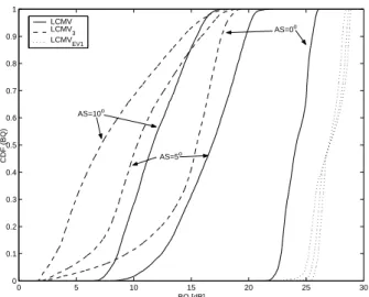
Figure 3 shows the comparison between the LCMV-based solutions for different AS values. As constraints we have considered: the mean DOAs (LMCV); 3 point constraints as depicted in Figure 1 (LCMV3); and one
EV constraint (LCMVEV1), obtained from a constraints
matrix formed by a 1◦ sampling over the angle
band-width. It can be noted that the increasing of AS causes LCMV and LCMV3 performance to decrease, while
LCMVEV1 performance remains practically unchanged.
0 5 10 15 20 25 30
0 0.1 0.2 0.3 0.4 0.5 0.6 0.7 0.8 0.9 1
BQ [dB]
CDF (BQ)
LCMV LCMV3 LCMVEV1
AS=10o
AS=5o
AS=0o
Figure 3: LCMV-based solutions performance compari-son for AS = 1◦,5◦and10◦.
The behavior of the LCMVEV faced with different
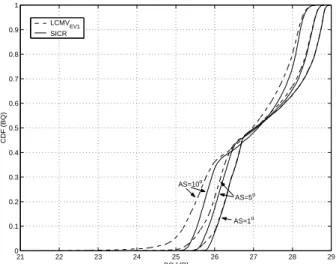
Finally, the SICR outperforms the LCMVEV1 for all
AS with a performance gap that increases with the AS, as shown in Figure 5.
5 CONCLUSIONS
An LCMV-based method for downlink beamforming was presented and compared with the SICR method. The method allows to consider the angular spread in the beamforming calculation, which is efficiently achieved by introducing eigenvector constraints in the optimiza-tion procedure. Moreover, a study into the number of constraints for the LCMV-based methods was provided. In fact, the performance of the point constrained beam-forming has shown to be strongly dependent on the num-ber of constraints, while the eigenvectorial method is much more robust. Besides, the best solution is achieved by the LCMV with only one eigenvector constraint.
When compared with the SICR, the LCMVEV1 has
shown a lower but satisfactory performance. Both meth-ods have approximately the same computational com-plexity due to the eigenanalysis for the SICR and the singular value decomposition for the LCMVEV1.
How-ever, the LCMVEV1solution is suitable for an adaptive
version while the SICR does not have one yet.
Then, a natural extension of this work is the investi-gation of the adaptive solution for LCMVEV1 in order
to reduce the computational burden, specially when the interferers position change.
Finally, an interesting aspect to proceed with the in-vestigation concerns the mathematical relations between both LCMC and SICR criteria. Clearly there is not a mathematical equivalence, but a number of situations where they present similar performance was verified. An interesting task seems to be the analytical derivation of the conditions for which such similarities hold.
References
[1] K. Hugl. Downlink beamforming using adaptive an-tennas. Diploma Thesis, Institut f¨ur Nachrichten-technik und HochfrequenzNachrichten-technik der Technischen Universit¨at Wien, Austria, May 1998.
[2] P. Zetterberg.Mobile Cellular Communications with Base Station Antenna Arrays: Spectrum Efficiency, Algorithms and Propagation Models. PhD thesis, Royal Institute of Technology, Stockholm, Sweden, 1997.
[3] T. Ast´e. M´ethodes de traitement d’antenne adaptatives pour un syst`eme de communications num´eriques radiomobiles de type GSM. PhD thesis, Conservatoire National des Arts et M´etiers, Paris, France, December 1998.
[4] L.S. Resende, J.M.T. Romano, and M.G. Bellanger. The Robust FLS Linearly-Constrained Algorithm:
An Improved Approach to Adaptive Spatial Filter-ing. InProceedings of ITS’94, pages 15–19, Rio de Janeiro - Brazil, August 1994.
[5] B.D. van Veen and K.M. Buckley. Beamforming: A versatile approach to spatial filtering. IEEE ASSP Magazine, pages 4–24, April 1988.
[6] K.M. Buckley. Spatial/Spectral Filtering with Lin-early Constrained Minimum Variance Beamformers.
IEEE Trans. on ASSP, 35(3):249–275, March 1987. [7] S. Haykin and A. Steinhardt, editors. Adaptive Radar Detection and Estimation. John Willey & Sons, New York, 1992.
5 10 15 20 25 30
0 0.1 0.2 0.3 0.4 0.5 0.6 0.7 0.8 0.9 1
BQ [dB]
CDF (BQ)
LCMVEV SICR
EV=1 EV=2 EV=3 EV=4
Figure 4: LCMVEVperformance for AS = 10◦ and
dif-ferent number of EV constraints.
21 22 23 24 25 26 27 28 29
0 0.1 0.2 0.3 0.4 0.5 0.6 0.7 0.8 0.9 1
BQ [dB]
CDF (BQ)
LCMVEV1
SICR
AS=1o AS=5o AS=10o
Figure 5: Comparison between the SICR and LCMVEV1