eve cccavalcante the use

2005 IEEE 6th Workshop on Signal Processing Advances in Wireless Communications

zyxwvutsrqponmlkjihgfedcbaZYXWVUTSRQPONMLKJIHGFEDCBA

THE

USE OF ORTHONORMAL BASES

zyxwvutsrqponmlkjihgfedcbaZYXWVUTSRQPONMLKJIHGFEDCBA

IN

EQUALIZATION STRUCTURES

zyxwvutsrqponmlkjihgfedcbaZYXWVUTSRQPONMLKJIHGFEDCBA

Ricardo

R.

zyxwvutsrqponmlkjihgfedcbaZYXWVUTSRQPONMLKJIHGFEDCBA

Araujo;

zyxwvutsrqponmlkjihgfedcbaZYXWVUTSRQPONMLKJIHGFEDCBA

GLrurd Favier; Joao C. M.

Mota; Charles

C.

Cavalcante

zyxwvutsrqponmlkjihgfedcbaZYXWVUTSRQPONMLKJIHGFEDCBA

rra@cefetce, br; favier Oi3s.unice.fr; mota@deti.ufc.br;

Charles

@

zyxwvutsrqponmlkjihgfedcbaZYXWVUTSRQPONMLKJIHGFEDCBA

gtel,ufc.br

ABSTRACT

In this work we propose the use of an ARMA equal- izer structured on generalized orthonormal bases for com- munication purposes. This equalizer structure presents a tapped line of all-pass and Iow-pass filters. Such a struc- ture is inherently stable since all its poles are within the unit circle. We also discuss a method for bases param- eterizing (poles choice) based on the channel characteris- tics. The proposed structure performances are compared with conventional FTR equalizer ones. The results are eval- uated in terms of MSE and overall numerical complexity. Traditional trained algorithms are employed for filter weight

adapting. Our simulations show that the proposed struc- ture leads to enhanced performances offering an alterna- tive reduced complexity solution for communication chan- nel equalization problem.

1. INTRODUCTION

The fact that IIR filters could be useful in adaptive signal processing has been widely explored in the last years. It is expected that these adaptive filters improve the perfor- mance of their FIR counterparts in many areas, as for exam- ple communication channel equalization.

The ARMA (Autoregressive Moving Average) structure

is adapted for IIR filtering, for the fact that its dynamics can

be represented by zeros and poles. Therefore, the aspects

of stability and convergence of the ARMA structure can be controlled from convenient criteria. The A N A filters can be implemented in several forms: blocks of coupled or de- coupled filters, in cascade, etc.

The so-called orthonormal filters such as Laguerre and Kautz filters form an other class of ARMA filters. Con- trarily to the conventional IIR filters, the orthonormal filters don’t have stability problems since theirs poles are inher- ently stables and can be defined by the user according to a

priori or posteriori knowledge of the channel.

Traditionally, the orthonormal bases are employed in

the context of system representation and identification prob- lems. The main motivation for using orthonormal bases in this context is the possibility to provide parsimonious repre- sentation

OF

systems by a strategy of fixing poles near where the poles of the underlying dynamics are believed to lie. This strategy leads to an improved accuracy representation of the systems using a reduced number of coefficients in the

filter as compared to conventional

zyxwvutsrqponmlkjihgfedcbaZYXWVUTSRQPONMLKJIHGFEDCBA

FIR

filters.

The equalizer complexity becpmes an important issue for its implementation in real time applications, principally in the future high capacity communications systems. That’s why a considerable amount of work is dedicated to the nu- merical complexity reduction of such structures. For this

sake, there are two principal ways for decreasing the com- putational cost of the equalizer sub-systems. We can work in the algorithm complexity bringing it more efficient or we can act in the equalizer structure in manner to obtain a reduction in the number of coefficients to adapt. It’s well known that there is a direct relationship between the num- ber of coefficients ( filter order) and the algorithm compu- tational cost. For instance, conventional LMS algorithm requires (3(hr) computations per sample while RLS need

( 3 ( N 2 ) per sample and DMI requires (3(N3) operations,

where N is the filter order.

In this work, we propose the use of ARMA filters based on the orthonorma1 functions in order to achieve a reduced complexity equalizer. The reduction in the computational cost is possible by decreasing the number of needed coeffi- cients to obtain a certain mean square error, There are sev- eral important reasons to consider orthonormal basis func- tions instead of the usual FIR implementations. First, the use of Laguerre or Kauts models (or more generally, or- thonormal basis functions) to describe the dynamical be- havior of a wide class of systems has been studied exten- sively in many works on system identification and control

f31, [41, [51, C6f. Second, the orthonormality property of

such a models offers many benefits in estimation problems, including better numerical conditioning of the data. Third, one of the primary motivations in using all-pass basis func- tions for adaptive filtering is the fact that it requires fewer parameters to model systems with long impulse responses.

In echo cancellation applications, for example, a long FIR

filter may be necessary to model the echo path and adaptive TLR techniques have been proposed as possible alternatives (e.g.,[l], [ 2 ] ) . These techniques are nevertheless known to face stability problems due to the arbitrary pole locations during filter operation.

In the following sections we describe how the orthonor- mal bases can be employed for the equalization problem. We put in evidence, through simulation results, the improved performances of the proposed structure, face to minimum and non-minimum phase channels, when compared to con-

ventional strategies. The rest of the paper is organized as follow; in section I1 we introduce the orthonormal bases. In section 111 we explain how the orthonormal-bases can be used for equalization. In section IV we describe a simple method for base choice. The results are compared to con- ventional structures in section V. Finally, we come with the

conclusions in section VI.

2. GENERALIZED ORTHONORMAL BASES

has an

zyxwvutsrqponmlkjihgfedcbaZYXWVUTSRQPONMLKJIHGFEDCBA

orthonormal bases. This fact is important because it

allows an unique representation of any element of the space

zyxwvutsrqponmlkjihgfedcbaZYXWVUTSRQPONMLKJIHGFEDCBA

as an orthonormal series expansion in terms of the elements

of

the Basis:

zyxwvutsrqponmlkjihgfedcbaZYXWVUTSRQPONMLKJIHGFEDCBA

i = l

where ci is a Fourrier coefficient determined as Q

zyxwvutsrqponmlkjihgfedcbaZYXWVUTSRQPONMLKJIHGFEDCBA

=

(z:

Bi).

It is clear that the representation in (1) is not useful in prac- tical problems where only a finite number of terms can be

handled. The solution is then to approximate 5 by a trucked

series like:

fig. 1. Stmcture

zyxwvutsrqponmlkjihgfedcbaZYXWVUTSRQPONMLKJIHGFEDCBA

of an N order GOE

zyxwvutsrqponmlkjihgfedcbaZYXWVUTSRQPONMLKJIHGFEDCBA

N

where 2 is an approximation of z.

Obviously the error decreases

zyxwvutsrqponmlkjihgfedcbaZYXWVUTSRQPONMLKJIHGFEDCBA

as the representation or-

der N increases. For a same representation order, the error

can vary according to the chosen orthonormal basis, i.e. an

orthonormal basis with similar dynamics provides better ap- proximation than other basis with different to 5 dynamics.

So, the basis choice plays a fundamental role in system rep-

resentation.

Consider the Hilbert space E’ formed by the sequences

f(n) with finite energy. The most common orthonormal basis on

C2

are the well known

FIR

basis that corresponds to the choice:

B . - --i

2 - 2

The use of FIR model structures to represent systems with long (possibly infinite) impulse responses has the dis-

advantage that the number of terms in the series expansion necessary to provide an acceptable approximation of the system is high and this may lead to poor accuracy in the estimated model.

Another well known bases are the Laguerre and Kautz

bases. The first one is well adapted for first order system representation while the second one is indicated for reso- nant systems. For systems with several resonant dynamics, more general orthonormal bases allowing the incorporation of prior information about several modes would be more desiderable. Examples of such more gcneral basis are the orthonormal basis generated by Inner Functions introduced by Heuberger, Van den Hof and co-workers or the gener- alized orthonormal basis with fixed poles studied by Nin-

ness and co-workers in [4]. The Kautz, Laguerre and

zyxwvutsrqponmlkjihgfedcbaZYXWVUTSRQPONMLKJIHGFEDCBA

FIR

model structures are all special cases of these methods.In this work, we consider the use of generalized orthonormal basis with fixed poles, henceforth called simply generalized orthonormal basis or GOB. The generalized orthonormal basis functions are built as follows:

where

zyxwvutsrqponmlkjihgfedcbaZYXWVUTSRQPONMLKJIHGFEDCBA

d = 0 or d

zyxwvutsrqponmlkjihgfedcbaZYXWVUTSRQPONMLKJIHGFEDCBA

1. Each p k , k = l , ..., i lpkl

<

1, is a basis

function pole. The factor

r d

doesn’t influence the base orthonormality. Its incorporation permits the strictly causal system representation.

3. THE UTILITY OF GOB FOR EQUALIZATION

In this paper we propose the use of equalization filters based on generalized orthonormal bases. The motivation of our proposition is to achieve an improved performance as com- pared to traditional

FIR

structures using lower order filters. This is possible due to GOB characteristics, which are well adapted for system identificationhepresentation. In fact, the main GOB virtue is its flexibility for the pole choice. In the equalization context, the problem can be stated as the identification of the channel transfer function inverse ( Zero Forcing approach) or the identification of a transfer func-

tion that minimizes some criterion (e.g. Minimum Square

Error criterion). The GOB based filter, hereafter called GOF (Generalized Orthonormal Filter), structure is illustrated in figure 1.

To obtain an efficient representation of a dynamical sys- tem using orthonormal expansion it is important that the ba- sis functions are calibrated to the underlying system charac- teristics. This gives increased rate of convergence of these expansions and hence accurate model with few parameters.

So, the basis choice is a fundamental point if we pretend

achieve an increased performance with GOF. Actually, a bad choice of the pole set that characterizes the GOB can leads to worst results when compared to FIR implemen- tations. That’s why an adaptive algorithm should be em- ployed to select the pole set that parameterizes the GOF. The stochastic gradient algorithms form, with no doubt, one

of the most popular class of adaptive algorithm due, prin- cipally, to their simplicity. However, the convergence of these algorithms is in8 uenced by the existence of local min- imums. This problem is observed even when just one pole

is adapted, e.g. for Laguere basis selection. Some authors have proposed other algorithms to accomplish this task, i.e. to select a pole set which optimizes the filter performances according to a certain criterion. The methods proposed in

[7], [ 8 ] , present a common point: they consider that all poles

are real. This consideration simplify an algorithm construc- tion, but it is not adequate for our case, since the presence of pairs of complex conjugate poles may be alIowed in order

N

zyxwvutsrqponmlkjihgfedcbaZYXWVUTSRQPONMLKJIHGFEDCBA

-

1

zyxwvutsrqponmlkjihgfedcbaZYXWVUTSRQPONMLKJIHGFEDCBA

zyxwvutsrqponmlkjihgfedcbaZYXWVUTSRQPONMLKJIHGFEDCBA

degree polynomial and ai = w , d n - . If the

Zero Forcing criterion is applied,

zyxwvutsrqponmlkjihgfedcbaZYXWVUTSRQPONMLKJIHGFEDCBA

h r e s ( z ) = 1.

Fig. 2.

zyxwvutsrqponmlkjihgfedcbaZYXWVUTSRQPONMLKJIHGFEDCBA

Channel identification.

4. THE BASIS CHOICE

In this paper we propose a simple method for the gener- alized orthonormal function pole selection. We divide the task in two parts. In the first one, we proceed with the chan- nel identification. In the second one, the poles are calcu-

lated according to the channel characteristics.

zyxwvutsrqponmlkjihgfedcbaZYXWVUTSRQPONMLKJIHGFEDCBA

In our work

we consider that the channel h ( z ) is modeled as an all zero

transfer function (MA model):

zyxwvutsrqponmlkjihgfedcbaZYXWVUTSRQPONMLKJIHGFEDCBA

L

h ( z ) = n ( z i - z )

zyxwvutsrqponmlkjihgfedcbaZYXWVUTSRQPONMLKJIHGFEDCBA

i = l

where L is the channel order.

Consider the chain formed by the transmitted symbols ~ ( n ) , the channel, the modified symbols z(n), the equalizer and the recuperated symbols y(n).

To recuperate the transmitted information, the equalizer must compensate the distortions produced by the channel. To do that, the channel zeros should be compensated by the equalizer poles. In our approach, the poles are determined according to the channel zeros. More precisely, we identify the channel in the first part of our method. The identifica-

tion procedure is accomplished using an ordinary FIR filter

as shown in fig.(2). A training sequence is employed for

the filter weight adjustments. After the training period the channel coefficients are estimated. We use this information to determine the channel order and to calculate the channel zeros. The DMI (Direct Matrix Inversion) algorithm is used for the channel identification.

In the second part, the zeros calculated are used to deter- mine each pole of the GOB. There are two possible scenar-

ios according to channel zero nature: minimum phase chan- nel and non-minimum phase channel. For each scenario we use a different strategy described as follows.

4.1. Minimum Phase Channel

When all the channel zeros are within the unit circle, our al- gorithm acts in a very simple way: for each zero zi we place

a pole pi where pi = zi.

zyxwvutsrqponmlkjihgfedcbaZYXWVUTSRQPONMLKJIHGFEDCBA

In this case, the filter is chosen to

be equal to the channel order. However, if we want, the filter order can be increased putting more poles in the origin, i.e.

the poles pi = 0

zyxwvutsrqponmlkjihgfedcbaZYXWVUTSRQPONMLKJIHGFEDCBA

V i

>

L, where 1; is the channel order. We

expect with this method to compensate each channel zero with a GOF pole. In a ideal case (perfectly channel iden- tification), if we choose N = L, we observe that the com- bined transfer function channel -F filter will be h r e s ( z ) = cy1Pl(z)

+

cr#~(z)

+.

..

+

c r ~ P ~ ( x ) , where

F'i(.z)

is an

4.2. Non-Minimum Phase Channel

For the non-minimum phase channel, the previous proce- dure must be rethinked. Indeed, for stability reasons the zeros outside the circle cannot be used as described before to select the GQF poles. Then, we divide the channel zeros in two categories: the zeros within the unit circle and the zeros outside the circle. For the zeros within the unit circle we place a correspondent pole in the same position. For the zeros outside the circle, we must use another approach. For each non-minimum phase zero we place a pole in the sym-

metrical point within the unit circle, i.e. pi = 1/25, This pair of zero/pole forms an all-pass filter. The all-pass filter created by the channel zero and the GOF pole will be re-

sponsible for a phase distortion. Then, we must use a phase correction network to overcome the all-pass filter effects. Such a procedure requires the realization of inverse all-pass systems. It is well known that an inverse transfer function of an all-pass filter can be approximated by a

FIR

filter. Let us discuss the problem of the

FIR

approximation of poles which is necessary for inverse all-pass modeling. Consider

the first order transfer function:

z

H ( z ) =

-

with lpi] 2 1

Z - P z

under the specific condition of the pole outside the unit cir- cle, H ( z ) can be described by the following series expan-

sion:

M

(4)

n=l

which converges since lpil

>

1. Thus the system can be in- terpreted as causal and non-stable or non-causa1 and stabIe. In the second case we get the impulse response:

n

h(n) -pi rn=1,2,3,

...

which can be approximated by an N order causal

FLR

zyxwvutsrqponmlkjihgfedcbaZYXWVUTSRQPONMLKJIHGFEDCBA

filter

by time truncation and shift. This causal impulse response can be written as:

N

n = 1

the second term describes N zeros in the z-plane, equidis- tantly spaced on a circle with the radius Ipil. One of these zeros (located at the position of the approximated pole) is canceled by the term H ( z ) . This form of approximation is based on a rectangular windowing of the true impulse re- sponse. Of course, this method can be applied for all-pass filter inversion.

Now, let us continue with the pole choice issue. Un- til this point, we proposed the placement of a GOF pole in the same position of each channel minimum phase zero and

a GOF pole in the symmetrical position for each channel

non-minimum phase zero. We have discussed about the use

all-pass fiIters formed

zyxwvutsrqponmlkjihgfedcbaZYXWVUTSRQPONMLKJIHGFEDCBA

by the pairs of non-minimum phase

zeros and their corresponding

zyxwvutsrqponmlkjihgfedcbaZYXWVUTSRQPONMLKJIHGFEDCBA

GOF poles, but how can

zyxwvutsrqponmlkjihgfedcbaZYXWVUTSRQPONMLKJIHGFEDCBA

we

combine the phase correction using

zyxwvutsrqponmlkjihgfedcbaZYXWVUTSRQPONMLKJIHGFEDCBA

FLR

filters and the GOF

pole choice? This can be accomplished in a very simple

way. First of all, we must remember that a FIR is a partic-

zyxwvutsrqponmlkjihgfedcbaZYXWVUTSRQPONMLKJIHGFEDCBA

ular case of a GOT; when all poles are placed in the origin. Then, the GQF structure can put into practice the channel zero compensation and the phase distortion correction tasks.

To do that, we mustjust place extra poles in the origin to im- plement a FIR. The all-pass inversion is accomplished using the GOF with a pertinent decision delay. The following ex-

ample illustrates our method. Consider a channel with zeros

zyxwvutsrqponmlkjihgfedcbaZYXWVUTSRQPONMLKJIHGFEDCBA

=

zyxwvutsrqponmlkjihgfedcbaZYXWVUTSRQPONMLKJIHGFEDCBA

{ZI 22

. . .

zizi+l

. .

. ZL). _where

zyxwvutsrqponmlkjihgfedcbaZYXWVUTSRQPONMLKJIHGFEDCBA

/ z k [

<

l , k = l ... i and

l z k l

>

Zk=-i+~ ... L . The GOF order is chosen to be N

>

L.

The GOF poles are chosen to be p j = zj for j

zyxwvutsrqponmlkjihgfedcbaZYXWVUTSRQPONMLKJIHGFEDCBA

= 1

.

.

. i and

pJ = 1/$ f o r j = i + l .

.

. 1.

zyxwvutsrqponmlkjihgfedcbaZYXWVUTSRQPONMLKJIHGFEDCBA

F o r j = L + l _ _ .

N

p ,

zyxwvutsrqponmlkjihgfedcbaZYXWVUTSRQPONMLKJIHGFEDCBA

= 0.

The number of extra poIes in the origin (Le. the correction

phase FIR order) will increase as the number of all-pass fil- ters to inverse increases. In our simulations, the decision delay i s chosen to match the central

FlR

tap, that is, the de-

lay 6 = ( N

-

L ) / 2 ' . A more detailed description of this

method is available in [9].

Channel id. I Channel zeros

1

t

J -0.63 -0.95 0 0.2 0.2 0.3 0.5 0.95

I

1

2 I -0.7 -0.3 0.&+0.8i 0.8-0% 0.9

3

I

0.5 0.7 1 1.1

4

I

-1i l i -0.86+0.51 0.86-0.53

Table 1. Channel zeros.

5. PERFORMANCE EVALUATION

Fig. 3. FIR and GOF performances. Channel 1

In this section the GOF performances are evaluated and com- pared with the conventional

FIR

structures. Both approaches are compared under two aspects: mean square error and computational cost. For the filter weight adjustments we employed two traditional trained algorithms: LMS and Di- rect Matrix Inversion. In each case, we use the same pa-

rameters ( adapting step, training sequence, input sequence, etc.) for the two approaches.

Initially, we consider a noiseless channel. In these con- ditions the channel identification can be realized without problems. In a second moment, the simulations are real- ized in a channel with Additive White Gaussian Noise. In

this case, the channel identification will not be perfect. As

consequence, the channel zeros estimation will be less ac- curate. The channel zero estimation accuracy influences the performances of the GOF equalizer.

In our simulations, we use the BPSK modulation and we consider that the transmitted data are identically distributed random variable with zero mean and unit variance, follow- ing the BPSK modulation alphabet. The channel identifica- tion is accomplished using the DMI algorithm. A training sequence of 64 symbols is employed in this task.

5.1. Noiseless Channel

In this subsection, we compare the FIR and GOF perfor- mances in different channels. The first one is a minimum phase channel, the second one is a non-minimum phase chan-

nel and the two others have zeros on the unit circle. The

zeros of each channel are presented in Tab.(l),

In fig (3) and (4), we show the simulation results for

channel I and 2 respectively. These simulations show us the

square error evolution when a LMS algorithm is employed for filter weight adjustment. In fig(3) the order of both fil-

ters is N = 8. In fig(4) the order is N = 7. We observe that,

'The optimal delay determination i s out of scope of his work.

in the same conditions, the GOF performances are superior

to the FIR performances in both channels. Indeed, The

FIR

reaches the GOF performances when the FIR order is in- creased to N = 90 for the channel 1 and,N = 150 for the channel 2.

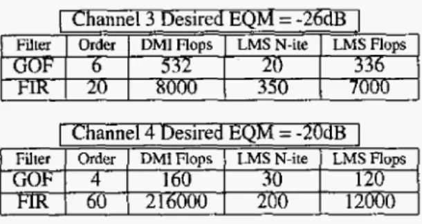
Now, we compare the computational cost of the two fil- ters. For a given performance in terms of EQM we compare the filter order required to reach the desired EQM. We also

compare the number of floating point operations needed for each case. For the GOF filter, we consider the computa- tional cost for the channel identification plus the computa- tional cost for the channel equalization. The LMS and DMI

algorithms are used. In the LMS algorithm, the number of iterations (N-ite) that leads the desired performance is also illustrated. The results are showed in Tab(2).

l

l

j

Filter

zyxwvutsrqponmlkjihgfedcbaZYXWVUTSRQPONMLKJIHGFEDCBA

I

zyxwvutsrqponmlkjihgfedcbaZYXWVUTSRQPONMLKJIHGFEDCBA

Order

I

zyxwvutsrqponmlkjihgfedcbaZYXWVUTSRQPONMLKJIHGFEDCBA

DMIFlops

I

LMSN-ite

1

LMSFlops

GOF I

zyxwvutsrqponmlkjihgfedcbaZYXWVUTSRQPONMLKJIHGFEDCBA

6 I 532 I 20 I 336

Filter Order DMI Flops LMS N-ite

zyxwvutsrqponmlkjihgfedcbaZYXWVUTSRQPONMLKJIHGFEDCBA

- G o P T ~~ 160 30

zyxwvutsrqponmlkjihgfedcbaZYXWVUTSRQPONMLKJIHGFEDCBA

FIR

60 2 16000 260

LMS Flops 120 12000

~

6. CONCLUSIONS

We have proposed a new equalizer filter structure based on generalized orthonormal bases. We also have presented an experimental method for basis parameterizing. The simula- tion results show us that the GOF structure presents better performances. in terms of EQM as compared to

FIR

struc- tures with the same order. For the same performance, the GOF structure presents a reduced computational cost due to the fewer coefficient number as compared to the traditional FIR solutions. Nevertheless, our results were obtained in stationary channels. In this condition, the basis parameter- izing must be accomplished once during the equalization process. If the channel changes during the equalization, the poles of bases should be updated. According to our method, the pole updating requires a new channel identi- fication. That is why the proposed method is suitable for packet data transmission systems, where a training sequence is generally employed for equalization purposes.

Table 2. Computational cost comparative.

7. REFERENCES

Fig. 5.

zyxwvutsrqponmlkjihgfedcbaZYXWVUTSRQPONMLKJIHGFEDCBA

Channel zero estimation.

zyxwvutsrqponmlkjihgfedcbaZYXWVUTSRQPONMLKJIHGFEDCBA

S N R = 3dB.

zyxwvutsrqponmlkjihgfedcbaZYXWVUTSRQPONMLKJIHGFEDCBA

5.2. Noisy Channel

It is well known that the noise influences the second order statistics based algorithms. So, this is the case of the DMI algorithm used in the first stage, the channel identification, of our method. Actually, the noise brings more difficult the correct channel identification and the zeros estimation. In the fig (5), we show the noise effect over the zero estima- tion. The simulation was realized using a S N R of 3dB. The circles represent the channel zeros and the @ represent the zero estimation. As the zero estimation plays a fundamen-

tal role in the GOF results, the overall filter performances decreases in the presence of noise. Nevertheless, the GOF performance remains greater than the FIR one. This is il- lustrated in fig(6). In this simulation, we compare the FIR

and GOF performances in terms of MSE as function of the

SNR. The filter order

zyxwvutsrqponmlkjihgfedcbaZYXWVUTSRQPONMLKJIHGFEDCBA

N = 8 and the channel 1 is employed

in the simulation.

(11 R. Merched and A. H. Sayed, “Extended fast fixed-

order RLS adaptive filters,” Proc. ISCAS, Sydney, Aus- tralia, May 2001.

P I

s.

Fiori “Blind Intrinsically- Stable 2-Pole n R Filtering” al url

w w . cifeseernj.nec. co~urtic~e/fioriO2bEind. hnnl,

2002.

[3] B.Wahlberg, System Identification using Laguerre models, IEEE Trans, Automat. Control., vol. 36, pp. 55 I - 562, May. 199 I .

[4] B. Ninness and E Gustafsson, “A Unifying Construc- tion of Orthonormal Bases for System Identification,”

IEEE, Transactions on Automatic Control , vol. 42, N

4,

pp. 515-521,1997.

[SJ

P.S.C. Heuberger; P.M.J. Van den Hof et O.H. Bosgra

, “A generalized orthonormal basis for linear dynamical systems” , IEEE, Transactiorzs on Automatic Control. ,

V. 40, N. 3, pp. 451465,1995.

161 T. A. Oliveira e Silva , “Sobre os Filtros de Kautz e sua

Utilizqso na Aproximago de Sistemas Lineares Invari- antes no Tempo”, PhD Thesis of Universidade de Aveiro,

Aveiro Portugal, 1994.

[7] B.E. Sarroukh, “Signal Analysis: representaion tools,”

Ph.D Thesis of University of Technology of Eindhoven,

Eindhoven, Holand, 2002.

[8]

N.

Tanguy; R. Morvan; P. Vilbt; L. C. Calvez, “Im- proved Method for Optimum Choice of Free Parameter in Orthogonal Approximations”, IEEE Trans. on Sign.

Process., vol. 47 , N 7, pp. 25762578,1999.

[9] RI R. de Araujo , “Traitement Spatio-Tempore1 Bas6 sur Lutilisation de Bases Orthonomales Gin6ralisCes : Ap- plication aux dseaux de paquets” , PhD Thesis of Uiii-