Analysis of injected apparent power and flicker in a distribution network after wind power plant connection

Published in IET Renewable Power Generation Received on 5th February 2007

Revised on 19th September 2007 doi: 10.1049/iet-rpg:20070059

ISSN 1752-1416

Analysis of injected apparent power and

flicker in a distribution network after wind

power plant connection

A.P. de Moura

*

A.A.F. de Moura

*

A.A.F. de Moura

*

Federal University of Ceara, Fortaleza, Ceara´, Brazil

*Wind Energy and Power System Laboratory, CEP-60810-110, Rua Francisco Farias Filho, Coco´ 230-602, Brazil E-mail: ailson@dee.ufc.br

Abstract: The maximum apparent power that can be injected in a bus and the flicker emission can represent a significant limit in the total capacity of a wind farm when wind turbines are connected to a radial distribution system. Quantification of these values is important in determining the largest number of wind turbines that can be connected in a network. The calculation of maximum apparent power and flicker of residential and commercial radial distribution feeder with remotely connected wind turbines has been investigated using elaborated specific software denominated winds port program and data from two energy systems. The developed software can calculate the approximate injected maximum apparent power, for a wind farm, in one bus of the network and in two buses of the network, simultaneously, without the need of a load flow program. The various simulations results reveal that wind farm capacities, in each bus, can be limited firstly for flicker and later for bus injected power for a voltage variation value, and the calculation of approximate apparent powers allows a precise and fast adjustment of voltage variation. If a load flow program is used for the determination of the wind farm maximum apparent power in each bus of the distribution system, a lot of simulations with a lot of attempts must be necessary. Therefore the methodology used by the authors is advantageous.

Nomenclature

Ef vector of fault voltages

E0 vector of prefault voltages

Zii element of the principal diagonal of the

bus impedance matrix

Zij element of the bus impedance matrix

zpk,pk impedance of the branch

2If vector of fault currents

zif ground impedance in the bus i

zk

f

ground impedance in the bus k Ei0 prefault voltage

Ii

f

fault current

Sn rated apparent power of the wind

turbine

Sk short-circuit power at the point of

common coupling (PCC)

c grid impedance phase angle

q phase angle between voltage and current

Pst short-term flicker emissions from the

wind turbine installation

Plt long-term flicker emissions from the

wind turbine installation

c(ck, va) flicker coefficient of the wind turbine for

the bus impedance phase anglec, at the PCC, and for the given annual average wind speed, va at hub-height of the

wind turbine at the site

Nwt number of wind turbines connected to

the PCC

kf(ck) flicker step factor

Kn(c) voltage change factor

N10,i

and

N120,i

TN turbines number

TNtrue true turbines number

EL emission level

P flicker emission from a single wind turbine during continuous operation

Smax maximum apparent power of the wind

farm

Stmax true maximum apparent power of the

wind farm

DV steady-state voltage change of the grid at the point of common coupling (normalised to nominal voltage)

DVtrue true steady-state voltage change of the

grid at the point of common coupling (normalised to nominal voltage)

Vcb voltage of base case

Vcwf voltage of case with wind farm

Vcwf-true voltage of case with true turbines

number

1

Introduction

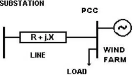
An important question, when installing wind turbines with the generator connected directly to the grid, is to quickly know what is the maximum injected wind power on determined bus of the radial distribution system. The injected wind power alters the voltage quality, and therefore this wind power must be limited. The ability of the grid to absorb disturbances is directly related to the short-circuit power level of the point in question. The short-circuit power level in a given point in an electrical network is a measure of its strength and, although not directly a parameter in the voltage quality, has a heavy influence [1]. Therefore the maximum apparent power injected in a bus is limited by short-circuit power of this bus. Another factor that contributes to a bad voltage quality is the flicker. Electrical flicker is a measure of voltage variations, which may cause disturbances to consumers [2].

This paper describes a study to determine the maximum apparent power injected in a bus and flicker of remotely embedded wind turbines in typical radial 11 kV distribution residential feeder and in typical radial distribution commercial feeder. Then, these values are used to calculate the maximum number of connected wind turbines in a bus. The radial distribution commercial feeder investigated operating within a 6% voltage band, and a residential feeder operating within more stringent voltage limits of +_{2%. The elaboration of specific software}

denominated winds port program allows to obtain the

maximum apparent power injected in the system and the flicker level in each bus quickly. The paper is organised in the following way; the used methodology is presented in Section 2. Section 3 presents the studied cases, and Section 4 presents the conclusions.

2

Methodology

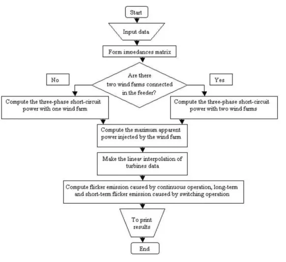
The methodology employed is based upon several simulations of wind farms integrated with the operation of the radial distribution system in heavy load. A software denominated winds port program was developed, and the procedure to determine the maximum apparent power and consequently the maximum number of wind turbines in each bus of the distribution system is the following: to calculate the short-circuit power of each bus with one or two wind farms connected in the networks at the same time; to establish the voltage variation, in steady state, allowed by energy company; to calculate the maximum apparent power that can be injected in each bus using algebraic equations; to divide the value of the maximum apparent power calculated by the value of the rated apparent power of the wind turbine; to establish a integer value for the number of wind turbines. Besides, the levels of flicker emission are calculated quickly, because they can limit the number of wind turbines. The short-circuit powers of the buses are calculated for the two simulated feeders that are a feeder with residential characteristic and another with commercial characteristic. A brief description of the developed software is provided below.

2.1 Winds port program

The winds port program processes together the data of the electric distribution system with the electric machines data of the wind farm to allow the necessary analysis. The winds port program (version 1.0) calculates the following parameters: the three-phase short-circuit power of each bus of the electric system, the equivalent impedances in module and angle, X/R

relationships, the maximum apparent power injected by wind farm that each bus supports for not surpassing the voltage variation value in the own bus, the flicker emission caused by wind farm during continuous operation, the long-term flicker emission caused by wind farm during switching operations, the short-term flicker emission caused by wind farm during switching operations and for the induction machines the voltages variations caused by inrush currents.

2.1.1 Impedance matrix: Winds port program forms the short-circuit matrix. The bus impedance matrix contains the impedances in the point of each bus in relation to an arbitrarily chosen bus. The impedance in the point of a bus is the equivalent between the impedance and the reference. The bus impedance matrix also contains the transfer impedance between each bus of the system and other buses, with relationship to the reference bus. Certain transfer impedances are starting from the calculation of the voltages in each one of the other buses of the system, with relationship to the reference, when a certain bus receives an injection

of unitary current. The short-circuit matrix is formed using the classic procedure by a step-by-step formation [3]. Certain assumptions in forming the bus impedance matrix are: (1) The passive network includes the impedances of all the circuit components. The nodes of interest are brought out of the bounded network, and it is excited by a unit generated voltage. (2) The network is passive in the sense that no circulating currents flow in the network. Also, the load currents are negligible with respect to the fault currents. For any currents an external path (a fault or load) must exist to flow. (3) All terminals that are marked 0 are at

Figure 1 Basic flow chart of winds port program

Figure 2 Step-by-step formation of bus impedance matrix a Adding a tree branch

the same potential. All generators have the same voltage magnitude and phase angle and are replaced by one equivalent generator connected between 0 and a node. For fault current calculations a unit voltage is assumed. During computer process, the following connections can occur: adding a tree branch to an existing node and adding a link as shown in Fig. 2 [4].

Adding a tree branch to an existing node: If there

is no coupling between pk and any existing branch xy, then

Z_kj ¼Z_pj j ¼1, 2,...,m j =k (1)

Zkk ¼Zpkþzpk,pk (2)

If the new branch is added betweenp and the reference node 0, then

Z_pj¼0 (3)

Z_kj¼0 (4)

Zkk¼zpk,pk (5)

Adding a link: A link node can be added as shown in

Fig. 2b. As k is not a new node of the system, the dimensions of the bus impedance matrix do not change; however, the elements of the bus impedance matrix change. To retain the elements of the primitive impedance matrix let a new node ‘e’ be created by breaking the link pk, as shown in

Fig. 2c.

If there is no mutual coupling between pkand other branches and p is the reference node

Z_pj¼0 (6)

Zej ¼ZpjZkj (7)

Zee ¼zpk,pkZke (8)

The artificial node can be eliminated using (9)

Z_bus,modified ¼Z_{bus,primitive}ZjeZ 0 je

Z_ee (9)

The equation that relates the bus impedance matrix with the injected currents and with the voltages in the buses is

shown in (10)

Ef1

Ef2

Efk

Efn 2 6 6 6 6 6 6 6 6 6 6 6 6 6 4 3 7 7 7 7 7 7 7 7 7 7 7 7 7 5 ¼

E01

E02

E0k

E0n 2 6 6 6 6 6 6 6 6 6 6 6 6 6 4 3 7 7 7 7 7 7 7 7 7 7 7 7 7 5 þ

Z11 Z12 Z1k Z1n

Z21 Z22 Z2k Z2n

Zk1 Zk2 Zkk Zkn

Zn1 Zn2 Znk Znn

2 6 6 6 6 6 6 6 6 6 6 6 6 6 4 3 7 7 7 7 7 7 7 7 7 7 7 7 7 5 0 0

_If_k

0 2 6 6 6 6 6 6 6 6 6 6 6 6 6 4 3 7 7 7 7 7 7 7 7 7 7 7 7 7 5 (10)

2.1.2 Calculation of short-circuit current and short-circuit power: The simultaneous short-circuit currents, in buses ‘i’ and ‘k’, can be calculated by (11) and (12) to proceed

If_i ¼ E

0

i(z

f

kþZkk)E

0

kZik

(zfkþZkk)(zfi þZii)Zik2

(11)

If_k¼ E

0

k(z

f

i þZii)E

0

iZik

(zf_kþZ_kk)(zf

i þZii)Zik2

(12)

The short-circuit power can be determined by (13)

Sk¼E0iIfi (13)

each PCC

DV₁

DV₂

DVn 2 6 6 6 6 4 3 7 7 7 7 5 ¼

jS_{max 1}j

jS_k1j cos(c1þq1) jS_{max 2}j

jS_k2j cos(c2þq2)

jS_maxnj

j_Sknj cos(cnþqn) 2 6 6 6 6 6 6 6 6 6 4 3 7 7 7 7 7 7 7 7 7 5 (14)

Only valid for cos(c_iþq_i).0:1

2.1.4 Flicker: Voltage variations caused by fluctuating loads and/or production are the most common cause of complaints over the voltage quality. Very large disturbances may be caused by melters, arc-welding machines and frequent starting of (large) motors. Slow voltage variations within the normal – 10þ6% tolerance band are not disturbing and neither are infrequent (a few times per day) step changes up to 3%, though visible to the naked eye. Fast and small variations are called flicker [1].

The 99th percentile flicker emission from a single wind turbine during continuous operation shall be estimated applying (15) below[5]

P_st¼P_lt¼c(c_k,v_a)Sn

S_k (15)

In case more wind turbines are connected to the PCC, the flicker emission from the sum can then be estimated

from (16) below [6]

P_stP¼P

ltP¼

1 Sk ffiffiffiffiffiffiffiffiffiffiffiffiffiffiffiffiffiffiffiffiffiffiffiffiffiffiffiffiffiffiffi X Nwt i¼1

(c(c_k,v_a)S_n)2

v u u

t (16)

The flicker emission because of switching operations of a single wind turbine shall be estimated by applying (17) and (18) below [7]

P_st¼18N0:31

10 kf(ck)

Sn

S_k (17)

P_lt ¼_8N0:31

120 kf(ck)

S_n

S_k (18)

In case more wind turbines are connected to the PCC, the flicker emission from the sum can then be estimated from (19) and (20) below [6]

P_stP ¼18

S_k

X Nwt

i¼1

N_10,i(k_f(c_k)S_n)3:2 !0:31

(19)

P_ltP ¼ 8

S_k

XNwt

i¼1

N_120,i(kf(ck)Sn)

3:2 !0:31

(20)

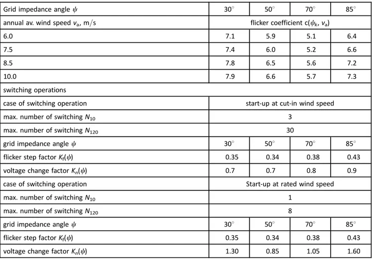
Flicker evaluation is based on IEC 61000-3-7 which gives guidelines for emission limits for fluctuating loads in medium voltage (MV, i.e. voltages between 1 and 36 kV) and high voltage (HV, i.e. voltages between 36 and 230 kV) networks. The recommended values are given inTable 1 [8].

In general, Plt should be smaller thanPst to consider

the fact that the irritability caused by the flicker is a cumulative effect that grows with the time.

3

Case studies

Two radial feeders are investigated: a commercial feeder operating within a+_{6% voltage band, and a residential}

feeder with more stringent voltage limits of+_{2%. The}

two radial feeders are presented in [9].

3.1 Residential feeder

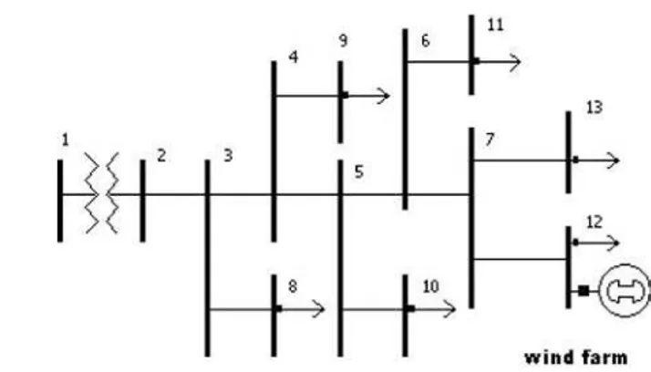
The 11 kV residential feeder is shown in Fig. 4. The feeder is supplied by a 3 MVA transformer. The transformer has a nominal on-load voltage ratio of 33/

11 kV and an associated impedance of 0.005þj0.006 pu. The feeder has a maximum demand of 1.89 MVA at a power factor of 0.95 lagging. Short-circuit power at bus 1, 33 kV is equal to Sk¼398 MVA. Details of the bus load and

connecting line data are given in [9, 10]. The load is

Figure 3 Wind farm connected with a radial distribution system

Table 1 Flicker planning and emission levels for medium voltage (MV) and high voltage (HV)

Flicker severity factor Planning levels Emission levels

MV HV MV and HV

Pst 0.9 0.8 0.35

modelled as constant impedance. The wind farms simulation in distribution system begins in bus 5 and it is going until the bus 13. The short-circuit power level in bus 5 until the bus 13 is shown inTable 2.

The grid impedance phase angle starting from bus 5 until the bus 13 is shown in Table 3.

The data of the power quality measurement of the wind turbine according to IEC61400-21 are presented in Table 4. Those data are supplied by wind turbine manufacturers, and they are used for the determination of the flicker emission levels (EL) in agreement with (15) – (20) [1]. The flicker coefficients, the flicker step factor and the voltage change factor from wind turbines are determined through a lineal interpolation between the values corresponding to the angles of 308_{, 50}8_{, 70}8 _{and 85}8_.

This procedure is made with an auxiliary subroutine that is a part of the winds port program. For the given case the annual average wind speed of the site of the wind farm at hub height of the turbines is 7.2 m/

s. Thus the wind speed class of 7.5 m/s is used. The type of wind turbine: staal, direct grid coupled induction generator. The wind turbine data are: rated power 600 kW, rated apparent power 607 kVA, rated voltage 609 V, rated current 508 A, max. power 645 kW, max. reactive power 114 kVAR.

3.1.1 Analysis of flicker and injected power: residential feeder: Fig. 5 shows the calculated values of wind turbine flicker emissions during continuous operation and wind turbine flicker emissions caused by switching operations. These values were calculated for the bus 5, the bus that presented the highest short-circuit power. In Fig. 5, the flicker ELs were calculated successively for a wind farm connected in bus 5 with one up to seven wind turbines. With seven wind turbines, the limit of flicker emission is larger than the limit allowed in the norm, as shown to proceed.

The graph shows that the values of flicker emission of wind turbines during continuous operation are smaller than the values of long-term flicker emissions. The values of short-term flicker emissions from wind turbines are already larger than the values of long-term flicker emissions. In agreement with

Table 1, the wind farm connected in bus 5 is limited in continuous operation (0.27) to a number of six turbines; in terms of Pst (0.34) ELs, the wind park is

not limited, and in terms of Plt (0.26) ELs, it is

limited to three turbines.

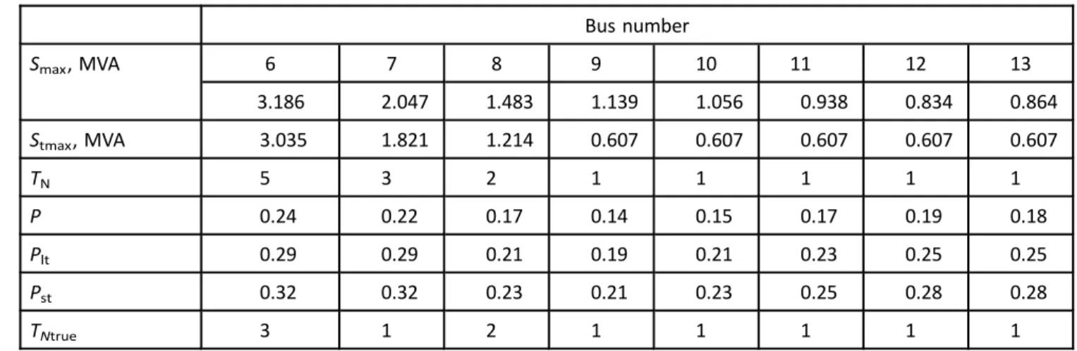
Fig. 6shows the short-circuit power in each bus, the calculated maximum apparent powers, and the true maximum apparent powers in buses 5 until 13. The true maximum apparent power (MVA) is multiple value of 0.607 (MVA), that is smaller, equal or approximately equal to the value of the maximum apparent power.

The graph shows that the maximum apparent power that can be injected in bus 5 is 4.234 MVA. This value corresponds to seven (4.234/

0.607¼ 6.98ffi7) turbines with a voltage variation

limit of 2%. Therefore as seen previously, the flicker limit restricts the injected power before the placement of seven turbines in the bus 5. Table 5

shows the results for the other distribution system buses.

Figure 4 Residential feeder

Table 2 Short-circuit powers of the grid

Bus number

Sk, MVA 5 6 7 8 9 10 11 12 13

31.8691 29.5416 25.2936 29.1422 25.4698 22.8776 21.1767 19.0532 19.3544

Table 3 Grid impedance angle at point of common coupling

Bus number

anglec,8 5 6 7 8 9 10 11 12 13

Table 5shows that the flicker ELs in the buses 6 and 7 limit firstly the wind farm capacity. Thus, two turbines of the buses 6 and 7 should be removed to decrease the flicker EL, causing decrease in the true maximum apparent power of the respective wind farm. Thus, the true number of turbines (TNtrue) is determined by the flicker limit.

The commercial load flow program anarede (network analysis) was used just for the verification

of the voltage variations in the buses, limited at 2%: (1) when the maximum apparent power is injected in its respective bus; (2) when the apparent power corresponding to the true number of turbines that is injected in the distribution system. The program anarede is marketed by the electric energy researches center (CEPEL), Brazil. The load flow is based in the Newton – Raphson method. Table 6 presents the results.

Table 4 Flicker

Grid impedance anglec 308 508 708 858

annual av. wind speedva, m/s flicker coefficient c(ck,va)

6.0 7.1 5.9 5.1 6.4

7.5 7.4 6.0 5.2 6.6

8.5 7.8 6.5 5.6 7.2

10.0 7.9 6.6 5.7 7.3

switching operations

case of switching operation start-up at cut-in wind speed

max. number of switchingN10 3

max. number of switchingN120 30

grid impedance anglec 308 508 708 858

flicker step factorKf(c) 0.35 0.34 0.38 0.43

voltage change factorKn(c) 0.7 0.7 0.8 0.9

case of switching operation Start-up at rated wind speed

max. number of switchingN10 1

max. number of switchingN120 8

grid impedance anglec 308 508 708 858

flicker step factorKf(c) 0.35 0.34 0.38 0.43

voltage change factorKn(c) 1.30 0.85 1.05 1.60

The first verification of the voltage variations in the buses is made comparing the base case voltages with the voltages of the case with wind farm. The difference of results should be of 2% or a close value to this value. The voltages (Vcb) of the base

case happen when the distribution system operates without connection to wind farms. The voltages of the case with wind farms happen when the distribution system operates with the connection of wind farms operating with its values of maximum individual apparent power. Table 6 shows that all the voltage variations are approximately the same to 2%.

The final verification of the voltage variations in the buses is made comparing the base case voltages with the voltages of the case with true wind farm (V cwf-true). The voltages of the case with true wind farms

happen when the distribution system operates with the connection of wind farms operating with its values of true turbines number. Table 6 shows that all the voltage variations are smaller than 2%.

3.2 Commercial feeder

The feeder has a nominal demand of 5.456 MVA at 0.85 p.f. lagging for a reference voltage of 11 kV or

1.0 pu. Details of the bus load and connecting line data are given in [9, 10]. The load is modelled as constant impedance. The 11 kV 12-bus commercial feeder is shown in Fig. 7. Short-circuit power at bus 1, 33 kV, is equal toSk¼398 MVA.

Several combinations of buses, two to two, were simulated. In each one of the buses, its maximum apparent powers were injected. The apparent powers are calculated through (11) – (14). Among those combinations, there are the buses 8 and 12. The power flows injected by the two wind farms do not cause violation of transport capacity in the lines or in the substation transformer.

Table 5 Short-circuit powers, true maximum apparent powers, turbines number and flicker in buses 6 until 13 Bus number

Smax, MVA 6 7 8 9 10 11 12 13

3.186 2.047 1.483 1.139 1.056 0.938 0.834 0.864

Stmax, MVA 3.035 1.821 1.214 0.607 0.607 0.607 0.607 0.607

TN 5 3 2 1 1 1 1 1

P 0.24 0.22 0.17 0.14 0.15 0.17 0.19 0.18

Plt 0.29 0.29 0.21 0.19 0.21 0.23 0.25 0.25

Pst 0.32 0.32 0.23 0.21 0.23 0.25 0.28 0.28

TNtrue 3 1 2 1 1 1 1 1

Table 6 Load flow program results

Bus number

Vcb, pu 5 6 7 8 9 10 11 12 13

0.999 0.997 0.994 1.007 1.001 0.995 0.992 0.989 0.989

Vcwf, pu 1.015 1.015 1.013 1.028 1.022 1.016 1.014 0.973 1.011

DV, % 1.6 1.8 1.9 2.1 2.1 2.1 2.2 1.6 2.2 Vcwf-true, pu 1.010 1.011 1.000 1.024 1.012 1.007 1.006 1.004 1.004 DVtrue, % 1.1 1.4 0.6 1.7 1.1 1.2 1.4 1.5 1.6

3.2.1 Analysis of flicker and injected power: commercial feeder: Figs. 8 and 9 show the flicker emission calculated for the buses 8 and 12. Figs. 8

and 9 show the calculated values of flicker emission of wind turbines during continuous operation and flicker emission of wind turbines caused by switching operations.

The graphs above show that in agreement with

Table 1, the wind farm connected in the bus 8 is limited in continuous operation (0.29) to a number of two turbines; in terms of Pst (0.32) ELs, the wind

farm is not limited and in terms of Plt (0.29) ELs, the

wind farm is limited to two turbines. Already for the bus 12 the wind farm is limited in continuous operation (0.28) to a number of three turbines; in terms of Pst (0.28) ELs, the wind farm is not limited

and in terms of Plt (0.26) ELs, it is limited to three

turbines.

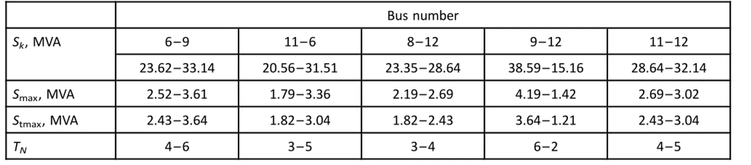
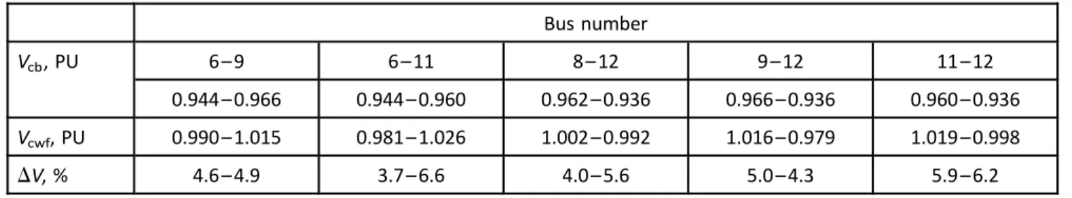
Table 7shows the simultaneous short-circuit powers in buses 6 and 9, 6 and 11, 8 and 12, 9 and 12 and 11 and 12, respectively, true maximum apparent powers of wind farm, the calculated maximum apparent powers and turbines number in the same buses. These bus combinations were chosen because the wind farms do not cause violation of transport capacity in the lines or in the substation transformer when connected in these buses. A load flow program results is shown inTable 8. The load flow verifies just the voltage variations in the buses, limited at 6%, when the maximum apparent power is injected in its respective bus.

Table 8 shows that the voltage variations are approximately close to the sought values. The determination of the approximate maximum apparent power allows to adjust precisely in the voltages variations. This verification procedure is done quickly. Being the case of the buses 8 and 12, the level of flicker emission limits the number of wind turbines in the buses 8 and 12, respectively, in 2 and 3 wind turbines. Thus, the new values of voltage variations in the buses 8 and 12 will be 2.6% and 4.0%, respectively. If there is reinforcement in the lines of the distribution system, the number of turbines will increase and the new values of voltage variation can be verified. The results of the simulations show that it is not always possible to obtain a voltage variation of 6% simultaneously in two buses. If a load flow is used to determine the turbine number in each wind farm simultaneously, starting from the base case, a lot of simulations will be necessary. The processing of load flow increases in the measure and in that increases the short-circuit power of the buses. In the case of the buses 6 and 9: TN-bus 6¼4, TN-bus 9¼6.

Theoretically, this corresponds for (1þ_{9) 9}/2¼45

Figure 8 Flicker emission: bus 8

Figure 9 Flicker emission: bus 12

Table 7 Apparent powers and turbines number – two simultaneous wind farms Bus number

Sk, MVA 6 – 9 11 – 6 8 – 12 9 – 12 11 – 12

23.62 – 33.14 20.56 – 31.51 23.35 – 28.64 38.59 – 15.16 28.64 – 32.14

Smax, MVA 2.52 – 3.61 1.79 – 3.36 2.19 – 2.69 4.19 – 1.42 2.69 – 3.02

Stmax, MVA 2.43 – 3.64 1.82 – 3.04 1.82 – 2.43 3.64 – 1.21 2.43 – 3.04

processings of load flow. Consider one wind farm with 20 turbines in 2 buses: this corresponds for (1þ₁₉₎

19/2¼190 processings of load flow. Thus, the

calculation of the approached apparent power values is advantageous.

4

Conclusions

This paper describes a study to determine the maximum bus injected apparent power and flicker of remotely embedded wind turbines in radial distribution systems. The determination of the maximum injected apparent power is limited at one or two wind farms connected simultaneously to the distribution system. The wind farm capacities, in each bus, can be limited firstly for flicker and later for bus injected power, for a voltage variation value, and the calculation of the approximate apparent powers allows a precise and quick voltage variation adjustment. If a load flow program is used, for the determination of the maximum apparent power of wind farm in each bus of the distribution system, a lot of simulations, with a lot of attempts, will be necessary until that the voltage variation in each bus is allowed by the energy company. The methodology proposed has the advantage to determine the maximum apparent power with only one calculation. It also determines the flicker ELs. Therefore the methodology presented in this paper is quite advantageous and can be a better tool for power systems planning in wind farms.

5

References

[1] DEUTSCHES WINDENERGIE INSTITUT: ‘Wind turbine grid connection and interaction’ (DEWI, UK, 2001)

[2] SCHLABBACH J, BLUME D, STEPHANBLOME T: ‘Voltage quality in electrical power systems’, IEE power series: no. 362001)

[3] BROWN HE: ‘Solution of large networks by matrix methods’ (John Wiley & Sons, 1975)

[4] DAS JC: ‘Power system analysis: short-circuit, load flow and harmonics’ (Marcel Decker, Inc., 2002)

[5] LARSSON A: ‘Flicker emission of wind turbines during continuous operation’, IEEE Trans. Energy Convers., 2002, 17, (1), pp. 114 – 118

[6] IEC61400-21: ‘Wind turbine generator systems – measurement and assessment of power quality characteristics of grid connected wind turbines’, 2001 [7] LARSSON A: ‘Flicker emission of wind turbines caused by switching operations’,IEEE Trans. Energy Convers. 2002,17, (1), pp. 119 – 123

[8] IEC61000-3-7:‘Electromagnetic compatibility (EMC) – part 3: limits – section 7: assessment of emission limits for fluctuating loads in MV and HV power systems – basic EMC publication’, 1996

[9] PERSAUD S,FOX B,FLYNN D: ‘Impact of remotely connected wind turbines on steady state operation of radial distribution networks’,IEE Proc., Gener. Transm. Distrib., 2000,147, (1), pp. 157 – 163

[10] CHIS M,SALAMA MMA,JAYAAAM S: ‘Capacitor placement in distribution systems using heuristic search strategies’, IEE Proc., Gener. Transm. Distrib., 1997, 144, (3), pp. 225 – 230

Table 8 Load flow program results: two simultaneous wind farms

Bus number

Vcb, PU 6 – 9 6 – 11 8 – 12 9 – 12 11 – 12

0.944 – 0.966 0.944 – 0.960 0.962 – 0.936 0.966 – 0.936 0.960 – 0.936 Vcwf, PU 0.990 – 1.015 0.981 – 1.026 1.002 – 0.992 1.016 – 0.979 1.019 – 0.998