ISSN 0101-8205 www.scielo.br/cam
The effect of the nonlinearity on GCV
applied to Conjugate Gradients in
Computerized Tomography
REGINALDO J. SANTOS1 and ÁLVARO R. DE PIERRO2 1Departamento de Matemática, ICEx, Universidade Federal de Minas Gerais
CP 702, 30123-970 Belo Horizonte, MG, Brazil
2Department of Applied Mathematics – IMECC, State University of Campinas CP 6065, 13081-970 Campinas, SP, Brazil
Emails: [email protected] / [email protected]
Abstract. We study the effect of the nonlinear dependence of the iteratexk of Conjugate Gradients method (CG) from the databin the GCV procedure to stop the iterations. We compare two versions of using GCV to stop CG. In one version we compute the GCV function with the iteratexkdepending linearly from the databand the other one depending nonlinearly. We have tested the two versions in a large scale problem: positron emission tomography (PET). Our results suggest the necessity of considering the nonlinearity for the GCV function to obtain a reasonable stopping criterion.
Mathematical subject classification: 62G05, 92C55, 65F10, 65C05.
Key words: Generalized Cross Validation, Tomography, Conjugate Gradients.
1 Introduction
We consider the problem of estimating a solutionx of
Ax+ǫ=b, (1.1)
where Ais a real m×n matrix,bis an m-vector of observations andǫ is an error vector. We assume that the components ofǫ are random with zero mean,
uncorrelated and with varianceσ2(unknown); i.e.;
Eǫ =0, Eǫǫt =σ2I, (1.2) whereE denotes the expectation andI is the identity matrix.
If A is a full rank matrix, the Gauss-Markov Theorem states that the least squares solution of (1.1), i.e., x˜ = (AtA)−1Atb, is the best unbiased linear estimator of x, meaning that it is the minimum variance estimator (see, for example [26]). But, if Ais ill-conditioned, this minimum variance is still large. It is well known that, if we allow the estimator to be biased the variance could be drastically reduced (see [28, 29]).
One way to do this, is by considering solutions of regularized problems of the form
minimize ||Ax−b||2+λxtB x , (1.3) for a positive real numberλ, whereBis ann×n matrix, that introducesa priori information on the problem. For example, Bcould be the matrix associated to the discretization of derivatives enforcing smoothness ofx.
Another way is to apply an iterative method that is convergent to the solution of
minimize ||Ax −b|| (1.4)
In this case, a regularization effect is obtained by choosing as ‘solution’ an early iterate of the method (See [31, 9] and the references therein, or see [14, Chapter 7]). Here the iteration numberk plays the role of the parameter λof the first approach. For stationary iterative methods in [10] and [23] it is shown that this approach is equivalent in some sense to the first one.
A crucial point in both approaches is the choice of the regularization parameter λin (1.3) or the iteration numberk in the second approach. A possibility is to approximate a value of λ, such that, the average of the mean square error is minimum, i.e.,λsolves the problem
minimize E T(λ) , (1.5)
where
T(λ)= 1
m||Ax−Axλ||
where xλ is the solution of (1.3) andx is one solution of (1.1). Probably, the
most popular of these methods is Generalized Cross-Validation (GCV) (See [33, 16]).
Ifxλis a estimator forx(the solution of (1.3) or one iterate of a iterative method
convergent to the solution of (1.4)), the influence operator Aλis defined as
Aλb= Axλ. (1.7)
For the solution of (1.3), the influence operator is given by
Aλb= A(AtA+λB)−1Atb (1.8)
IfAλ is given by (1.8), in [6, 13] the GCV functionV(λ)was defined as
V(λ)=
1
m||b−Axλ|| 2
1
mT r(I −Aλ)
2. (1.9)
GCV chooses the regularization parameter by minimizingV(λ). This estimate is a rotationally invariant version of Allen’s PRESS, or Cross-Validation [1].
In [6, 13] was proven that, ifAλis given by (1.8), then
|E T(λ)−E V(λ)+σ2|
E T(λ) <
2µ1+µ
2 1 µ2
µ21
(1−µ1)2 (1.10) whereµ1= m1TrAλµ2= m1TrA2λ, whenever 0< µ1<1. In [8] Eldén presents
a method to compute the trace-term of the GCV function using bidiagonaliza-tion. In [12], Golub and Von Matt proposed an iterative method to approximate the trace-term of the GCV function for large scale problems. In [21], Golub, Nguyen and Milanfar extended the derivation of the GCV function to under-determined systems with applications to superresolution reconstruction.
Another approach is to apply an iterative method directly to the least square problem
minimize ||Ax−b||2
stationary linear iterative methods. It is well known that the Conjugate Gradients method applied to the normal equations (CGLS) associated to the problem (1.1) can achieve its best accuracy significantly faster than stationary methods and that CGLS can be used as a regularizing algorithm (see [22]). However, the iterations of CG are a nonlinear function of the data vectorb, and, as pointed out in [15], a very good stopping rule should be used. In [15], Hanke and Hansen suggest a Monte Carlo GCV procedure to stop CGLS and the ν-method ([15], pages 298–299). But the nonlinearity of the influence operator in the case of CGLS is not taken into account. While for theν-method the influence operator is linear or affine, for CGLS it is nonlinear. However they observe that the application of their procedure “can suffer severely from the nonlinearity of CGLS”. Also in [15] another even more crude approximation is used. In the later case the denominator of the GCV functional is approximated by the expression1− n−p+k
m
2
, where pis the matrix rank; and this is the same for every value ofb([15], page 307).
The main goal of this paper is to compare a Monte Carlo GCV procedure deduced in Section 2 that takes into account nonlinearity with another one that linearizes the influence operator for large scale problems like that arising in Positron Emission Tomography (PET).
Another alternative to GCV can be the use of the L-curve (see [15]), that is not considered in this article because of the fact that we wanted to make explicit the importance of considering the nonlinear part of CG and because of the lack in that approach (the L-curve) of most of the statistical information provided by the problem.
In Section 2 we derive an inequality like (1.10), when Aλ is a nonlinear
2 GCV for a nonlinear influence operator
We would like to obtain a good estimate for
T(λ)= 1
m||Ax−Axλ||
2, (2.1)
using the relative residual defined by
U(λ)= 1
m||b−Axλ||
2 (2.2)
and our information on the error (1.2). The next result is a technical lemma.
Lemma 1. Let F(λ), g(λ), G(λ), r(λ)and H(λ)be real valued functions with λinRandαreal number. If
G(λ)= F(λ)+α(1−2g(λ))+r(λ) (2.3)
and
H(λ)= G(λ)
(1−g(λ))2, (2.4) then the following expression is valid:
H(λ)−F(λ)−α F(λ) =
1 (1−g(λ))2
−αg(λ)
2+r(λ)
F(λ) +2g(λ)−g(λ)
2 (2.5)
Proof. From (2.3) e (2.4) we have that
H(λ)−F(λ)−α F(λ)
= 1
(1−g(λ))2
F(λ)+α(1−2g(λ))+r(λ)
F(λ) −
(1−g(λ))2(F(λ)+α) F(λ)
= 1
(1−g(λ))2
1−αg(λ)
2
F(λ) −(1−g(λ))
2+ r(λ) F(λ)
,
(2.6)
Throughout this paper we will assume that the influence operator, defined by
Aλ(b)= Axλ, (2.7)
is a continuously differentiable operator as a function ofb, withbvarying in an open set, that containsAx, and if we denote byD Aλ(·)the Jacobian of Aλ(·),
we have the next result.
Proposition 2. Let{xλ}be a family of estimators for the solution of(1.1), and
(1.2). For eachλ, Aλ(·)is continuously differentiable in, then
EU(λ)= E T(λ)+σ2
1− 2
mT r(D Aλ(Ax))
+E(ǫtOλ(ǫtǫ)) , (2.8)
where U(λ)is given by(2.2), T(λ)by (2.1)and the function Oλ(ǫtǫ)is such
that||Oλ(ǫtǫ)|| ≤ Mǫtǫ, for some M >0.
Proof. Expanding the square of the residual of (1.1) and (1.6), atxλwe get that
||b−Axλ||2− ||Ax−Axλ||2 = ||Ax+ǫ−Axλ||2− ||Ax −Axλ||2 = ||ǫ||2+2ǫt(Ax−Axλ) .
(2.9)
Now, expanding Aλ(·)at Ax+ǫ around the point Axin Taylor formula:
Aλ(Ax+ǫ)=Aλ(Ax)+D Aλ(Ax)ǫ+Oλ(ǫtǫ) (2.10)
whereOλ(ǫtǫ)satisfies the hypothesis. Using (1.1) and (2.10) above we obtain
Axλ = Aλ(b)= Aλ(Ax+ǫ)= Aλ(Ax)+D Aλ(Ax)ǫ+Oλ(ǫtǫ) . (2.11)
Dividing (2.9) bym, applying the expectation and using (1.2), (2.11) we obtain
EU(λ) = E T(λ)+ 1
mE
||ǫ||2+ 2
m
EǫtAx−EǫtAxλ
= E T(λ)+σ2− 2
m
E
ǫtAλ(Ax)
+E
ǫtD Aλ(Ax)ǫ+EǫtOλ(ǫtǫ)
= E T(λ)+σ2 1− 2
mT r(D Aλ(Ax))
+E
ǫtOλ(ǫtǫ),
Let we introduce the GCV function for nonlinear influence operators. For Ax ∈, we define the GCV functional by
V(λ)=
1
m||b−Axλ|| 2
1
mT r(I −D Aλ(Ax))
2, (2.13)
In spite of the fact that we do not know the value of Ax, we will show bellow how we can obtain a good approximation for the denominator of (2.13) for large scale problems.
Theorem 3. Let{xλ} be a family of estimators for the solution of (1.1), for
which(1.2)is valid. and for V(λ)given by(2.13)the following equality holds
E V(λ)−E T(λ)−σ2 E T(λ)
= 1
(1−µ1(λ))2
−σ2µ1(λ)2+r(λ)
E T(λ) +2µ1(λ)−µ1(λ) 2 ,
(2.14)
whereµ1(λ)= 1
mT r(D Aλ(Ax))and r(λ)=E(ǫ tO
λ(ǫtǫ)).
Proof. By Proposition 2 the inequality (2.8) holds. Applying Lemma 1 we
get (2.14).
The next Proposition is the basis of our approximation scheme.
Proposition 4. Let w = (w1, . . . , wm) be a vector of random components with normal distribution, that is, w ∼ N(0,Im×m). Suppose that Aλ(·) is continuously differentiable in the open setthat contains Ax . Let x1λand x2λthe estimators corresponding to the data vectors b+δwand b−δwrespectively. Then
E
wt[w−A(xλ
1 −x2λ)/2δ] wtw
= 1
mT r(I −D Aλ(Ax))+E
wtOλ(ǫtǫ+2δ|ǫtw| +δ2wtw)
wtw
Proof. Expanding Aλ(·)at Ax+ǫ+δwand Ax+ǫ+δwaround the point
Axup to the first order:
Ax1λ = Aλ(Ax+ǫ+δw)
= Aλ(Ax)+D Aλ(Ax)(ǫ+δw)+Oλ
(ǫ+δw)t(ǫ+δw) (2.16)
and
Ax2λ = Aλ(Ax+ǫ−δw)
= Aλ(Ax)+D Aλ(Ax)(ǫ−δw)+Oλ
(ǫ−δw)t(ǫ−δw). (2.17)
Thus, we obtain
Ax1λ−Ax2λ
2δ =D Aλ(Ax)w+Oλ(ǫ
tǫ+2δ|ǫtw| +δ2wtw) (2.18) and the result follows using a slight extension of the Theorem 2.2 of [11].
For the sake of consistency with the usual mathematical notation for the it-erations of an algorithm, in what follows, the parameter λwill be substituted byk.
3 Monte Carlo Implementation of GCV for Conjugate Gradients
Our main goal in this section is to apply our Monte Carlo Implementation of GCV as stopping rule for Conjugate Gradients method for solving (1.1). Now, each iteratexk is an estimate of the solution of (1.1) andk plays the role ofλ. In Section 2 we showed that GCV is applicable to influence operators that are continuously differentiable in an open set that contains Ax.
The Conjugate Gradients method of Hestenes and Stiefel [3] applied to the normal equations (CGLS) can be written as: (for a givenx0)
r0=b−Ax0, s0 =Atr0, w0=s0 and for k =0,1, . . . pk = Awk
αk = ||s
k||2
rk+1=rk−αkpk sk+1= Atrk+1 βk = ||s
k+1||2
||sk||2
wk+1=sk+1+βkwk
For eachk >0, the operatorT(k)(b)= xk is nonlinear and it is continuously differentiable outside the termination set (closed)
Mk=
b∈Rm|PR(A)b−Ax0is a linear combination ofkeigenvectors ofA At
,
where PU denotes the orthogonal projection onto the subspace U (i.e., = (Rn−Mk)). IfAis an ill-conditioned operator, thenT(k)(·)is discontinuous in Mk−1, as pointed out by Eicke, Louis and Plato in [7] in the infinite dimensional
context. The same arguments of [7] can be easily used to understand the behavior of the method in the discrete case. Forb in Mk−1, we definebl = b+σl
1 2ul,
whereulis the singular vector associated to the singular valueσl. From the fact thatbl ∈ Mkit follows that
||T(k)(b)−T(k)(bl)|| = ||A†b−A†bl|| = 1
σ
1 2
l .
Thus, ifσl ≈0, then||T(k)(b)−T(k)(bl)|| ≈ ∞. And ifb∈ Mk−1andbwisb
perturbed by a random vectorw, we should also have||T(k)(b)−T(k)(bw)|| ≈ ∞. But, usually in ill-posed problems the vectorb has all the components of the singular vectors. It means thatb does not belong to a termination set Mk, for anyk.
Taking into account the results of the preceding section we describe the algo-rithm for calculating an approximation of the GCV functional (2.13) by using central differences to approximate the direcional derivative.
Algorithm 1.
(i) Generate a pseudo-random vectorw =(w1, . . . , wm)t ∈Rm from a nor-mal distribution with standard deviation equal to one, i.e.,
(ii) For eachk, compute the iteratesxk xk
1 andx2k corresponding tob,b−δw eb+δw, respectively, whereδ=10−4. Take
NL(k)=
wt[w−A(xk
1−x2k)/2δ] wtw
2
, (3.19)
as an approximation for1
mT r[Im−D Ak(Ax)]
2
;
(iii) For eachktake
VNL(k)= 1
m||b−Ax k||2
NL(k) (3.20)
4 Positron emission tomography
The goal of positron emission tomography (PET) is the quantitative determina-tion of the moment-to-moment changes in the chemistry and flow physiology of radioactive labelled components inside the body. The mathematical problem consists of reconstructing a function representing the distribution of radioactivity in a body cross-section from measured data that are the total activity along lines of known location. One of the main differences between this problem and that arising in X-ray tomography [17] is that here measurements tend to be much more noisy, so, direct inversion using convolution backprojection (CBP) doesn’t necessarily give the best results (see [30]).
In positron emission tomography (PET) [27], the isotope used emits positrons which annihilate with nearly electrons generating two photons travelling away from each other in (nearly) opposite directions; the number of such photons pairs (detected in time coincidence) for each line or pair of detectors is related to the integral of the concentration of isotope along the line.
Suppose now that we discretize the problem by subdividing the reconstruction region inton small square-shaped picture elements (pixels, for short) and we assume that the activity in each pixel j is a constant, denoted by xj. If we countbicoincidences alongmlines andai jdenotes the probability that a photon emitted by pixel j is detected by pair i, then yi is a sample from a Poisson distribution whose expected value isn
j=1ai jxj.
of Conjugate Gradients to the system (4.21) could give similar or better results [24] and it is a reasonable example to test the capability of GCV as a stopping rule for CG.
With the objetive of comparing the GCV procedures in Computerized To-mography we apply the Conjugate Gradients method “preconditioned” with a symmetric ART (from algebraic reconstruction technique) method, as presented recently in [24], i.e. we apply CG to solve the generalized least squares problem (CGGLS)
min||Cω−1(b−Ax)||2. whereCω =(D+ωL)D−
1
2, ifA At =L+D+Lt, whereLis the strictly lower
triangular part andDthe diagonal of A At respectively. This corresponds to apply CG to the system
AtCω−tCω−1Ax = AtCω−tCω−1b, (4.1) In the ART method,ωis the relaxation parameter. Here it has a different role, it is the weight of the lower triangular part ofAin the preconditioning. Whenω is zero, this corresponds to a diagonal scaling.
The Conjugate Gradients method applied to (4.21) can be written as:
r0 = Cω−1(b−Ax0), s0 =AtCω−tr0, w0=s0 and for k =0,1, . . . pk = Cω−1Awk
αk = ||s
k||2
||pk||2 xk+1 = xk+αkwk rk+1 = rk−αkpk sk+1 = AtCω−trk+1 βk = ||s
k+1||2 ||sk||2
wk+1 = sk+1+βkwk
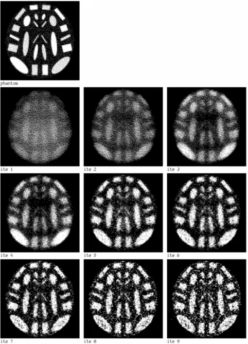
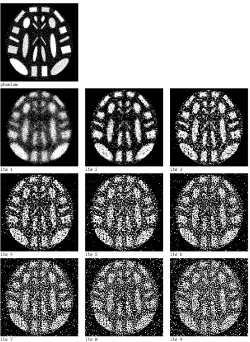
In our numerical experiments we used the programming system SNARK93, developed by the Medical Image Processing Group of the University of Penn-sylvania [5]. The images to be reconstructed (phantom) were obtained from a computerized atlas based on typical values inside the brain, as in [18]. The data collection geometry was a divergent one simulating a typical PET data acqui-sition [5]. We used a discretization withn =95×95 pixels and the divergent
geometry had 300 views, of 101 rays each, a total number ofm =30292
equa-tions (8 rays were not considered because their lack of intersection with the image region). The starting point was a uniform imagex0=(a, . . . ,a)t, where ais an approximation of the average density of the phantom given by
a =
m
i=1bi
m i=1
n j=1ai j
. (4.2)
The choice of a uniform non-zero starting point was advocated by L. Kaufman [20] and it is widely accepted as the best choice for many researchers in PET. The vectorbwas taken from a pseudorandom number generator with a Poisson distribution (see [19]). The total photon count was 2 022 085, 991 179, 514 925 and 238 172 (monotonically increasing noise).
We have performed experiments applying Algorithm 1 with photon counts 2 022 085, 991 179, 514 925 and 238 172 and with six values ofω, between 0.0 and 0.025. For each valueωand each photon count we repeated the experiments ten times. The ten tests gave very similar results.
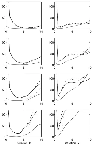
We plotted, for one of the tests, in Figure 1 the functions
100 1 952||x
k−x||2
, 1
30292||Ax
k−Ax||2
, VMC−100 and VHH−100 against the iteration numberk, forω=0.0 (diagonal scaling) andω=0.025. Here we callVHHthe Monte Carlo GCV function, if we suppose that PCCGLS is a linear function of the data vectorb, as proposed by Hanke-Hansen in [15]. As expected, the minimum of our Monte Carlo GCV functionVMC(k)coincides with that of||A(xk−x)||2, and also the curves are very similar. We can see that
0 5 10 0
50 100
0 5 10
0 50 100
0 5 10
0 50 100
0 5 10
0 50 100
0 5 10
0 50 100
0 5 10
0 50 100
0 5 10
0 50 100
iteration, k
0 5 10
0 50 100
iteration, k
Figure 1 – Loss functions for the method CGGLS with ω = 0.0 (diagonal scaling) (left) and ω = 0.025 (right). The rows 1-4 correspond to 2 022 085, 991 179, 514 925 and 238 172 photon counts, respectively. The solid thin lines correspond to 1009512||xk−x||2; the thick ones, to 302921 ||Axk−Ax||2; the dashed lines to transla-tions ofVMCand dotted ones to translations ofVHH, i.e., if we suppose that CGGLS is
5 Concluding remarks
Iterative methods in Emission Computed Tomography, like RAMLA [4], that are being used nowadays by PET scanners (see for example http: / / www. medical.philips.com/us/products/pet/products/cpet/), are fast and produce high quality pictures (because they take into account the Poisson nature of the noise) in few iterations. So it was not our goal in this paper to compare Conjugate Gradient with those methods, but to show that our approximation of GCV is applicable as a stopping rule to the Conjugate Gradient method for large scale ill-posed problems, similar to Positron Emission Tomography (very large scale, not severely ill-posed and relatively large noise in the data). Some authors (see, for example, [15, 9]) have suggested the use of other approximations to GCV. Our experimental results show (Fig. 1) that Algorithm 1 gives very good (much better than Hanke et al’s) approximations for the minimum of||A(xk−x)||2.
Further research is needed to extend these applications of GCV to more gen-eral nonlinear methods and nonlinear problems. We also need more specific asymptotic theoretical results.
Acknowledgements. We are grateful to J. Browne and G.T. Herman for their
support on the use of SNARK93.
Álvaro R. De Pierro was partially supported by CNPq Grant No. 300969 / 2003-1 and FAPESP Grant No. 2002 / 07153-2, Brazil.
REFERENCES
[1] D.M. Allen, The relationship between variable selection and data augmentation and a method for prediction.Technometrics,16(1) (1974), 125–127.
[2] A. Björck and T. Elfving, Accelerated projection methods for computing pseudoinverse solutions of systems of linear equations.BIT,19(1979), 145–163.
[3] Åke Björck,Numerical Methods for Least Squares Problems. SIAM, Philadelphia (1996). [4] J. Browne and A.R. De Pierro, A row-action alternative to the em algorithm for maximizing
likelihoods in emission tomography.IEEE Trans. Med. Imag.,15(1996), 687–699. [5] J.A. Browne, G.T. Herman and D. Odhner, SNARK93 a programming system for image
[6] P. Craven and G. Wahba, Smoothing noisy data with spline functions.Numer. Math.,31(1979), 377–403.
[7] B. Eicke, A.K. Louis, and R. Plato, The instability of some gradient methods for ill-posed problems.Numer. Math.,58(1990), 129–134.
[8] L. Eldén, A note on the computation of the generalized cross-validation function for ill-conditioned least squares problems.BIT,24(1984), 467–472.
[9] H. Engl, M. Hanke and A. Neubauer,Regularization of inverse problems. Kluwer Academic Publishers Group, Dordrecht (1996).
[10] H.E. Fleming, Equivalence of regularization and truncated iteration in the solution of ill-posed image reconstruction problems.Linear Algebra and its Appl.,130(1990), 133–150. [11] D.A. Girard, A fast ‘Monte-Carlo cross-validation’ procedure for large least squares problems
with noisy data.Numer. Math.,56(1989), 1–23.
[12] G. Golub and U. von Matt, Generalized cross-validation for large-scale problems.Journal of Computational and Graphical Statistics,6(1997), 1–34.
[13] G.H. Golub, M.T. Heath and G. Wahba, Generalized cross-validation as a method for choosing a good ridge parameter.Technometrics,21(1979), 215–223.
[14] M. Hanke,Conjugate Gradient Type Methods for Ill-Posed Problems. Longman Scientific & Technical, Essex,UK (1995).
[15] M. Hanke and P.C. Hansen, Regularization methods for large-scale problems. Surv. Math. Ind.,3(1993), 253–315.
[16] P.C. Hansen,Rank-Deficient and Discrete Ill-Posed Problems. SIAM, Philadelphia (1998). [17] G.T. Herman,Image Reconstruction from Projections: The Fundamentals of Computerized
Tomography. Academic Press, New York (1980).
[18] G.T. Herman and L.B. Meyer, Algebraic reconstruction techniques can be made computa-tionally efficient.IEEE Trans. Med. Imaging,12(1993), 600–609.
[19] G.T. Herman and D. Odhner, Performance evaluation of an iterative image reconstruc-tion algorithm for positron emission tomography. IEEE Trans. Med. Imaging,10(1991), 336–346.
[20] L. Kaufman, Implementing and accelerating the EM algorithm for positron emission tomog-raphy.IEEE Trans. Med. Imag.,6(1987), 37–51.
[21] N. Nguyen, P. Milanfar and G. Golub, Efficient generalized cross-validation with applications to parametric image restoration and resolution enhancement. IEEE Transactions on Image Processing,10(9) (2001), 1299–1308.
[23] R.J. Santos, Equivalence of regularization and truncated iteration for general ill-posed problems.Linear Algebra and its Appl.,236(1996), 25–33.
[24] R.J. Santos, Preconditioning conjugate gradient with symmetric algebraic reconstruction technique (ART) in computerized tomography.Applied Numerical Mathematics,47(2003), 255–263.
[25] R.J. Santos and A.R. De Pierro, A cheaper way to compute generalized cross-validation as a stopping rule for linear stationary iterative methods.Journal of Computational and Graphics Statistics,12(2003), 417–433.
[26] S.D. Silvey,Statistical Inference. Penguin, Harmondsworth (1970).
[27] M.M. Ter-Pogossian et al., Positron emission tomography. Scientific American, October: 170–181, 1980.
[28] A. van der Sluis and H.A. van der Vorst, Numerical solution of large, sparse linear alge-braic systems arising from tomographic problems. In G. Nolet, editor,Seismic Tomography. D. Reidel Pub. Comp., Dordrecht, The Netherlands (1987).
[29] A. van der Sluis and H.A. van der Vorst, SIRT and CG type methods for the iterative solution of sparse linear least squares problems.Linear Algebra and its Appl.,130(1990), 257–303. [30] Y. Vardi, L.A. Shepp and L. Kaufman, A statistical model for positron emission tomography.
J. Amer. Stat. Assoc.,80(389) (1985), 8–37.
[31] C. Vogel,Computational methods for inverse problems. SIAM, Philadelphia (2002). [32] G. Wahba, Three topics in ill-posed problems. In H. Engl and C. Groetsch, editors,Inverse
and Ill-Posed Problems. Academic Press, New York (1987).