ISSN 0101-8205 / ISSN 1807-0302 (Online) www.scielo.br/cam
The global convergence of a descent
PRP conjugate gradient method
MIN LI1∗,∗∗, HEYING FENG2 and JIANGUO LIU1
1Department of Mathematics and Applied Mathematics, Huaihua University, Huaihua, Hunan 418008, P.R. China
2School of Energy and Power Engineering, Huazhong University of Science and Technology Wuhan, Hubei 430074, P.R. China
E-mail: [email protected]
Abstract. Recently, Yu and Guan proposed a modified PRP method (called DPRP method)
which can generate sufficient descent directions for the objective function. They established the global convergence of the DPRP method based on the assumption that stepsize is bounded away from zero. In this paper, without the requirement of the positive lower bound of the stepsize, we prove that the DPRP method is globally convergent with a modified strong Wolfe line search. Moreover, we establish the global convergence of the DPRP method with a Armijo-type line search. The numerical results show that the proposed algorithms are efficient.
Mathematical subject classification: Primary: 90C30; Secondary: 65K05.
Key words: PRP method, sufficient descent property, modified strong Wolfe line search,
Armijo-type line search, global convergence.
1 Introduction
In this paper, we consider the unconstrained problem
min f(x), x ∈ Rn, (1.1) #CAM-307/10. Received: 12/XII/10. Accepted: 17/IV/11.
*Corresponding author
where f : Rn → R is continuously differentiable. Nonlinear conjugate gradi-ent methods are efficigradi-ent for problem (1.1). The nonlinear conjugate gradigradi-ent methods generate iterates by letting
xk+1=xk+αkdk, k =0,1,∙ ∙ ∙ , (1.2)
with
dk = (
−g0, if k =0,
−gk+βkdk−1, if k ≥1,
(1.3) whereαk is the steplength,gk =g(xk)denote the gradient of f atxk, andβk is a suitable scalar.
Well-known nonlinear conjugate method include Fletcher-Reeves (FR), Polak-Ribière-Polyak (PRP), Hestenes-Stiefel (HS), Conjugate-Descent (CD), Liu-Story (LS) and Dai-Yuan (DY) [1–7]. We are particularly interested in the PRP method in which the parameterβkis defined by
βkPRP= g
T k yk−1
kgk−1k2
.
Here and throughout, k ∙ k stands the Euclidean norm of vector and yk−1 = gk −gk−1. The PRP method has been regarded as one of the most efficient conjugate gradient methods in practical computation and studied extensively.
Now let us simply introduce some results on the PRP method. The global con-vergence of the PRP method with exact line search has been proved by Polak and Ribière [3] under strong convexity assumption of f. However, Powell con-structed an example which showed that the PRP method with exact line searches can cycle infinitely without approaching a solution point [8]. Powell also gave a suggestion to restrictβk = max{βkPRP,0} to ensure the convergence. Based on Powell’s work, Gilbert and Nocedal [9] conducted an elegant analysis and showed the PRP method is globally convergent ifβkPRP is restricted to be non-negative and the steplength satisfies the sufficient descent condition gT
kdk ≤
−ckgkk2 in each iteration. In [10], Zhang, Zhou and Li proposed a three term PRP method. They calculatedkby
dk = (
−g0, if k=0,
−gk+βkPRPdk−1−θkyk−1, if k≥1,
whereθk = gT
kdk−1
kgk−1k2. It is easy to see from (1.4) that d
T
kgk = −kgkk
2. Zhang, Zhou and Li proved that this three term PRP method convergent globally with a Armijo-type line search.
In [11], Yu and Guan proposed a modified PRP conjugate gradient formula:
βkDPRP =
gkTyk−1
kgk−1k2
−tkyk−1k 2gT
kdk−1
kgk−1k4
, (1.5)
wheret >1/4 is a constant. In this paper we simply call it DPRP method. This modified formula is similar to the well-known CG_DESCENT method which was proposed by Hager and Zhang in [13]. Yu and Guan has proved that the directionsdk generated by the DPRP method can always satisfied the following sufficient descent condition
gkTdk ≤
1 4t −1
kgkk2. (1.6) In order to obtain the global convergence of the algorithm, Yu and Guan [11] considered the following assumption: there exists a positive constantα∗such that
αk > α∗holds for all indicesk. In fact, under this assumption, if the sufficient descent conditiongT
kdk ≤ −ckgk2is satisfied, the conjugate gradient methods with Wolfe line search will be globally convergent.
In this paper, we focus on the global convergence of the DPRP method. In Section 2, we describe the algorithm. The convergence properties of the algo-rithm are analyzed in Section 3 and 4. In Section 5, we report some numerical results to test the proposed algorithms by using the test problems in the CUTEr [23] library.
2 Algorithm
From the Theorem 1 in [11] we can obtain the following useful lemma directly.
Lemma 2.1. Let{dk}be generated by
dk = −gk+τdk−1, d0= −g0. (2.1) If gT
Proof. The inequality (1.6) holds forτ =βkDPRPfrom the Theorem 1 in [11]. For anyτ ∈(βkDPRP,max{0, βkDPRP}], it is clear thatβkDPRP ≤τ ≤0. IfgT
kdk−1≥ 0, then (1.6) follows from (2.1). IfgT
kdk−1<0, then we get from (2.1) that gkTdk = −kgkk2+τgkTdk−1≤ −kgkk2+βkDPDPg
T kdk−1≤
1 4t −1
kgkk2.
The proof is completed.
Lemma 2.1 shows that the directions generated by (2.1) are sufficient descent directions and this feature is independent of the line search used. Especially, if set
dk = −gk+βDPRPk dk−1, d0= −g0, (2.2)
βDPRPk =maxβkDPRP, ηk , ηk =
−1
kdk−1kmin{η,kgk−1k}
, (2.3) whereη >0 is a constant, it follows fromηk <0 that
βDPRPk =max
βkDPRP, ηk ∈
βkDPRP,max
0, βkDPRP .
So, the directions generated by (2.2) and (2.3) are descent directions due to Lemma 2.1. The update rule (2.3) to adjust the the lower bound onβkDPRP was originated in [13].
Now we present concrete algorithm as follows.
Algorithm 2.2. (The DPRP method) [11]
Step 0. Given constantε >0and x0∈ Rn. Set k :=0; Step 1. Stop ifkgkk∞≤ε;
Step 2. Compute dk by(2.2);
Step 3. Determine the steplengthαk by a line search;
It is easy to see that Algorithm 2.1 is well-defined. We analyse the conver-gence in the next sections. We do not specify the line search to determine the steplengthαk. It can be exact or inexact line search. In the next two sections, we devote to the convergence of the Algorithm 2.1 with modified strong Wolfe line search and Armijo-type line search.
3 Convergence of Algorithm 2.1 under modified strong Wolfe line search
In this section, we prove the global convergence of the Algorithm 2.1. We first make the following assumptions.
Assumption 3.1.
(I) The level set
= {x ∈ Rn : f(x)≤ f(x0)}
is bounded.
(II) In some neighborhood N of, function f is continuously differentiable and its gradient is Lipschitz continuous, namely, there exists a constant L >0such that
kg(x)−g(y)k ≤ Lkx−yk, ∀x,y ∈ N. (3.1) From now on, throughout this paper, we always suppose this assumption holds. It follows directly from the Assumption 3.1 that there exist two pos-itive constantsB andγ1such that
kxk ≤ B and kg(x)k ≤γ1, ∀x ∈. (3.2) In the later part of this section, we will devote to the global convergence of the Algorithm 2.1 under a modified strong Wolfe line search which determine the steplengthαk satisfying the following conditions
f(xk+αkdk)≤ f(xk)+δαkgkTdk,
|g(xk+αkdk)Tdk| ≤minM, σ|gkTdk| ,
where 0 < δ ≤ σ < 1 and M > 0 are constants. The purpose of this modi-fication is to make |gT
kdk−1| ≤ M always hold with the given M. Moreover, we can set M to be large enough such that min{M, σ|gT
kdk|} = σ|gkTdk|hold for almost all indicesk. At first, we give the following useful lemma which was essentially proved by Zoutendijik [19] and Wolfe [20, 21].
Lemma 3.2. Let the conditions in Assumption3.1hold,{xk}and{dk}be gener-ated by Algorithm 2.1 with the above line search, then
∞
X
k=0
(gT kdk)2
kdkk2 <+∞. (3.4)
Proof. We get from the second inequality in (3.3)
σgkTdk ≤gkT+1dk ≤ −σgkTdk, (3.5) From the Lipschtiz condition (3.1), we have
(σ−1)gTkdk ≤(gk+1−gk)Tdk ≤ Lαkkdkk2. Then
αk ≥
(σ −1)
L gT
kdk
kdkk2 =
(1−σ )
L
|gT kdk|
kdkk2. (3.6) Since f is bounded below and the gradient g(x)is Lipschitz continuous, from the first inequality in (3.3) we have
−
∞
X
k=0
αkgkTdk ≤ +∞. (3.7) Then the Zoutendijik condition (3.4) holds from (3.6) and (3.7). The following lemma is similar to the Lemma 4.1 in [9] and the Lemma 3.1 in [13], which is very useful to prove that the gradients cannot be bounded away from zero.
Lemma 3.3. Let the conditions in Assumption3.1hold,{xk}and{dk}be gener-ated by Algorithm2.1with the modified strong Wolfe line search. If there exists a constantγ >0such that
then
dk 6=0, ∀k ≥0, and ∞
X
k=0
kuk−uk−1k2<∞, (3.9) where uk =dk/kdkk.
Proof. Since kgkk > γ > 0, it follows from (1.6) that dk 6= 0 for eachk. We get from (3.4) and (1.6)
∞
X
k=0
γ4
kdkk2 ≤ ∞
X
k=0
kgkk4 kdkk2 ≤
4t 4t−1
2 ∞ X
k=0
(gkTdk)2
kdkk2 <∞, (3.10) wheret> 14 is a constant. Here, we define:
βk+=max{βDPRPk ,0}, βk−=min{βDPRPk ,0}, (3.11) rk = −gk+β
− k dk−1
kdkk , δk =β
+ k
dk−1
kdkk. (3.12)
By (2.2), (3.11) and (3.12), we have uk = dk
kdkk =
−gk+(βk++βk−)dk−1
kdkk =rk+δkuk−1.
Since theuk are unit vectors,
krkk = kuk−δkuk−1k = kδkuk−uk−1k. Sinceδk >0, we have
kuk−uk−1k ≤ k(1+δk)(uk−uk−1)k
≤ kuk−δkuk−1k + kδkuk−uk−1k
= 2krkk.
(3.13)
We get from the definition ofβDPRPk
krkkkdkk = k −gk+βk−dk−1k
≤ kgkk −min
βDPRPk ,0 kdk−1k
≤ kgkk −ηkkdk−1k
≤ kgkk + 1
kdk−1kmin{η, γ}
kdk−1k
≤ γ1+ 1 min{η, γ}.
Settingc=γ1+min{1η,γ} and combing (3.13) with (3.14), we have
kuk−uk−1k2 ≤(2krkk)2≤ 4c2
kdkk2. (3.15) Summing (3.15) overkand combing with the relation (3.10), we have
∞
X
k=0
kuk−uk−1k2≤ ∞
X
k=0 4c2
kdkk2 <∞.
The proof is completed.
Now we state a property for βDPRPk in (2.2), which is called Property(*) proposed by Gilbert and Nocedal in [9].
Property(*). Suppose that Assumption3.1and inequality(3.8)hold. We say that the method has Property(*) if there exist constant b > 1andλ > 0 such that
|βk| ≤b,
ksk−1k ≤λ⇒ |βk| ≤2b1,
(3.16) where sk−1=xk−xk−1=αk−1dk−1.
Lemma 3.4. If the modified strong Wolfe line search is used in Algorithm2.1, then the scalarβDPRPk satisfies the Property(*).
Proof. By the definition ofβDPRPk in (2.2), we have
|βDPRPk | ≤ |βkDPRP|, ∀k ≥0.
Under the Assumption 3.1, if (3.8) holds, we get from (3.3) and (1.6)
|βDPRPk | ≤ |β DPRP k |
≤ |g
T k yk−1|
kgk−1k2
+tkyk−1k 2|gT
kdk−1|
kgk−1k4
≤ kgkkkyk−1k kgk−1k2
+tkyk−1k 2M
kgk−1k4
≤ 2γ
2 1
γ2 +t 4γ12M
γ4 .
Ifsk−1< λ, then
|βDPRPk | ≤ |βkDPRP|
≤ kgkkkyk−1k kgk−1k2
+tkyk−1k 2M
kgk−1k4
≤
γ1
γ2 +t 2γ1M
γ4
kyk−1k
≤
γ1
γ2 +t 2γ1M
γ4
Lksk−1k.
(3.18)
(3.17) together with (3.18) implies the conditions in Property(*) hold by setting b = 2γ
2 1
γ2 +t 4γ12M
γ4 and λ=
γ1
Lb2. (3.19)
The proof is completed.
LetN∗denote the set of positive integer set. Forλ >0 and a positive integer
△, we define the index set:
Kk,λ△:=i ∈ N∗:k ≤i≤k+ △ −1,ksi−1k> λ . (3.20) Let|Kk,λ△|denote the number of elements inKk,λ△. We have the following Lemma which was essentially proved by Gilbert and Nocedal in [9].
Lemma 3.5. Let xk and dk be generated by Algorithm 2.1 with the modified strong Wolfe line search. If(3.8)holds, then there exists a constantλ >0such that for any△ ∈N∗and any index k0, there is an index k>0such that
|Kk,λ△|> △
2. (3.21)
The proof of Lemma 3.5 is similar to that of the Lemma 4.2 in [9], so we omit here. The next theorem, which is modification of Theorem 4.3 in [9], shows that the proposed Algorithm 2.1 is globally convergent.
Theorem 3.6.Let the conditions in Assumption3.1hold, and{xk}be generated by Algorithm2.1with the modified strong Wolfe line search(3.3), then either
kgkk =0for some k or
lim inf
Proof. We suppose for contradiction that both
kgkk 6=0 and lim inf
k→∞ kgkk 6=0. Denoteγ =inf{kgkk :k ≥0}. It is clear that
kgkk ≥γ >0, ∀k ≥0. (3.23) Therefore the conditions of Lemma 3.3 and 3.5 hold. Make use of Lemma 3.4, we can complete the proof in the same way as Theorem 4.3 in [9], so we omit
here too.
4 Convergence of the Algorithm 2.1 with a Armijo-type line search
In this section, we will prove the global convergence of the Algorithm 2.1 under an Armijo-type line search which determine
αk =max
ρj, j =1,2,∙ ∙ ∙
satisfying
f(xk +αkdk)− f(xk) <−δ1αk2kdkk 4
, (4.1)
whereδ1>0 andρ ∈(0,1).
We get from the definition of Algorithm 2.1 that the function value sequence
{f(xk)}is decreasing. And what’s more, if f is bounded from below, from (4.1) we have
∞
X
k=0
αk2kdkk4<∞ or ∞
X
k=0
αkkdkk2<∞. (4.2) Under Assumption 3.1, we have the following useful lemma.
Lemma 4.1. Let the conditions in Assumption3.1hold,{xk}and{dk}be gener-ated by Algorithm2.1with the above Armijo-type line search. If there exists a constantγ >0such that
kgkk> γ , ∀k ≥0, (4.3) then there exists a constant T >0such that
Proof. By the definition ofdkand the inequalities (3.1) and (3.2), we have
kdkk ≤ kgkk + |βkDPRP|kdk−1k
≤ kgkk +kgkkkyk−1kkdk−1k kgk−1k2
+tkyk−1k
2kgkkkdk −1k
kgk−1k4
kdk−1k
≤ γ1+
γ1Lαk−1kdk−1k2
γ2 +t
2γ12Lαk−1kdk−1k2
γ4 kdk−1k.
(4.2) implies thatαkkdkk2 →0 ask → ∞. Then for any constantb ∈ (0,1), there exist a indexk0such that
2tγ12Lαk−1kdk−1k2
γ4 <b, ∀k >k0. Then
kdkk ≤γ1+
γ2b 2tγ1
+bkdk−1k =c+bkdk−1k, ∀k>k0, wherec=γ1+ γ
2b
2tγ1 is a constant. For anyk >k0we have
kdkk ≤c(1+b+b2+ ∙ ∙ ∙ +bk−k0+1)+bk−k0kdk 0k ≤
c
1−b + kdk0k.
We can get (4.4) by setting
T =max{kd1k,kd2k,∙ ∙ ∙,kdk0k,
c
1−b + kdk0k}. Based on Lemma 4.6 we give the next global convergent theorem for Algo-rithm 2.1 under the above Armijo-type line search.
Theorem 4.2. Let the conditions in Assumption 3.1 hold, {xk} be generated by Algorithm2.1with the above Armijo-type line search, then eitherkgkk =0 for some k or
lim inf
k→∞ kgkk =0. (4.5) Proof. We suppose for the sake of contradiction thatkgkk 6= 0 for allk ≥ 0 and lim infk→∞kgkk 6=0. Denoteγ =inf{kgkk :k ≥0}. It is clear that
At first, we consider the case that lim infk→∞αk > 0. From (4.2) we have lim infk→∞kdkk = 0. This together with (1.6) gives lim infk→∞kgkk = 0, which contradicts (4.6).
On the other hand, if lim infk→∞αk = 0, then there exists a infinite index setK such that
lim inf
k∈K,k→∞αk =0 (4.7) The Step 3 of the Algorithm 2.1 implies thatρ−1αkdoes not satisfy (4.1). Namely
f(xk+ρ−1αkdk)− f(xk) >−δ1ρ−2αk2kdkk 4
. (4.8)
By the Lipschitz condition (3.1) and the mean value theorem, there is a
ξk ∈ [0,1], such that
f(xk+ρ−1αkdk)− f(xk)
= ρ−1αkg(xk+ξkρ−1αkdk)Tdk
= ρ−1αkgkTdk+ρ −1
αk(g(xk+ξkρ−1αkdk)−gk)Tdk
≤ ρ−1αkgkTdk+Lρ −2α2
kkdkk 2. This together with (4.8), (4.4) and (1.6) gives
4t−1 4t kgkk
2≤ −gT
kdk ≤αkρ−1(δ1kdkk4+Lkdkk2)
≤αkρ−1(δ1T4+L T2).
(4.9)
(4.7) and (4.9) imply that lim infk∈K,k→∞kgkk = 0. This also yields contra-diction, then the proof is completed.
5 Numerical results
The PRP+ code was obtained from Nocedal’s web page at
http://www.ece.northwestern.edu.nocedalsoftware.html
and the CG_DESCENT code from Hager’s web page at
http://www.math.ufl.edu/∼hager/papers/CG. All codes were written in Fortran77 and ran on a PC with 2.8 GHZ CPU processor and 2GB RAM mem-ory and Linux (Fedora 10 with GCC 4.3.2) operation system. We stop the iter-ation ifkgkk∞≤10−6or the total number of iterations is larger than 10000.
We tested all the unconstrained problems in CUTEr library [23] with their defaultdimensions. By the end of 2010, there were 164 unconstrained optim-ization problems in the CUTEr library. Moreover, five of them failed to install on our system for the limit storage space.
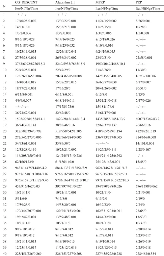
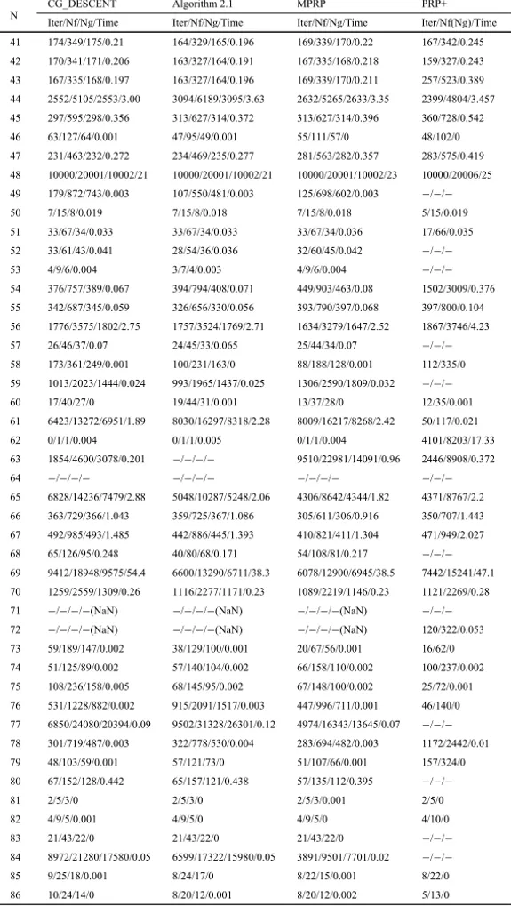
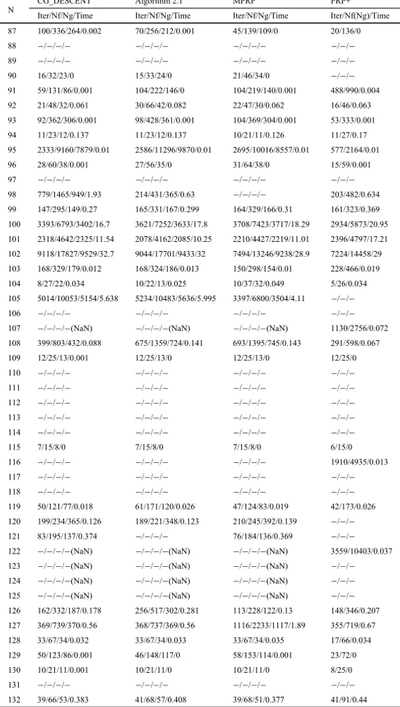
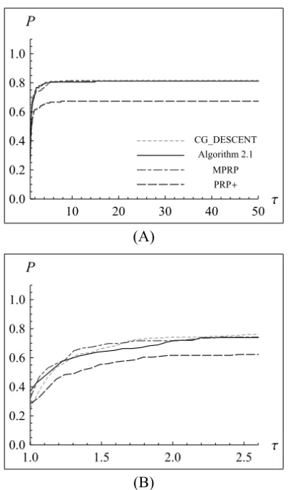
In order to get relatively bettert value in Algorithm 2.1, we tested the prob-lems witht = 0.3, 0.5, 0.7, 0.9, 1.1, 1.3, 1.5. We obtained from the data that Algorithm 2.1 witht=1.3 performed slightly better than others. So in this sec-tion, we only compare the numerical results for Algorithm 2.1 witht =1.3 with CG_DESCENT, MPRP and PRP+ method. The problems and their dimensions are listed in Table 1. Table 2 list all the numerical results, which include the total number of iterations (Iter), the total number of function evaluations (Nf), the total number of gradient evaluations (Ng), the CPU time (Time) in seconds, respectively. In Table 2, “−” means the method failed and “NaN” means that the cost function generated a “NaN” for the function value.
N Problem Dim N Problem Dim N Problem Dim
1 3PK 30 54 EIGENALS 110 107 OSBORNEA 5
2 AKIVA 2 55 EIGENBLS 110 108 OSBORNEB 11
3 ALLINITU 4 56 EIGENCLS 462 109 OSCIPATH 15 4 ARGLINA 200 57 ENGVAL1 5000 110 PALMER1C 8
5 ARGLINB 200 58 ENGVAL2 3 111 PALMER1D 7
6 ARGLINC 200 59 ERRINROS 50 112 PALMER2C 8
7 ARWHEAD 5000 60 EXPFIT 2 113 PALMER3C 8
8 BARD 3 61 EXTROSNB 1000 114 PALMER4C 8
9 BDQRTIC 5000 62 FLETCBV2 5000 115 PALMER5C 6
10 BEALE 2 63 FLETCBV3 100 116 PALMER6C 8
11 BIGGS6 6 64 FLETCHBV 100 117 PALMER7C 8
12 BOX 1000 65 FLETCHCR 1000 118 PALMER8C 8
13 BOX3 3 66 FMINSRF2 5625 119 PENALTY1 1000
14 BRKMCC 2 67 FMINSURF 5625 120 PENALTY2 200 15 BROWNAL 200 68 FREUROTH 5000 121 PENALTY3 100
N Problem Dim N Problem Dim N Problem Dim 16 BROWNBS 2 69 GENHUMPS 5000 122 PFIT1LS 3
17 BROWNDEN 4 70 GENROSE 500 123 PFIT2LS 3
18 BROYDN7D 5000 71 GROWTHLS 3 124 PFIT3LS 3
19 BRYBND 5000 72 GULF 3 125 PFIT4LS 3
20 CHAINWOO 4000 73 HAIRY 2 126 POWELLSG 5000
21 CHNROSNB 50 74 HATFLDD 3 127 POWER 10000
22 CLIFF 2 75 HATFLDE 3 128 QUARTC 5000
23 COSINE 10000 76 HATFLDFL 3 129 ROSENBR 2
24 CRAGGLVY 5000 77 HEART6LS 6 130 S308 2
25 CUBE 2 78 HEART8LS 8 131 SBRYBND 100
26 CURLY10 1000 79 HELIX 3 132 SCHMVETT 5000
27 CURLY20 1000 80 HIELOW 3 133 SCOSINE 100
28 CURLY30 1000 81 HILBERTA 2 134 SCURLY10 100 29 DECONVU 61 82 HILBERTB 10 135 SCURLY20 100
30 DENSCHNA 2 83 HIMMELBB 2 136 SCURLY30 100
31 DENSCHNB 2 84 HIMMELBF 4 137 SENSORS 100
32 DENSCHNC 2 85 HIMMELBG 2 138 SINEVAL 2
33 DENSCHND 3 86 HIMMELBH 2 139 SINQUAD 5000
34 DENSCHNE 3 87 HUMPS 2 140 SISSER 2
35 DENSCHNF 2 88 HYDC20LS 99 141 SNAIL 2
36 DIXMAANA 3000 89 INDEF 5000 142 SPARSINE 1000 37 DIXMAANB 3000 90 JENSMP 2 143 SPARSQUR 10000 38 DIXMAANC 3000 91 KOWOSB 4 144 SPMSRTLS 4999 39 DIXMAAND 3000 92 LIARWHD 5000 145 SROSENBR 5000 40 DIXMAANE 3000 93 LOGHAIRY 2 146 TESTQUAD 5000 41 DIXMAANF 3000 94 MANCINO 100 147 TOINTGOR 50 42 DIXMAANG 3000 95 MARATOSB 2 148 TOINTGSS 5000 43 DIXMAANH 3000 96 MEXHAT 2 149 TOINTPSP 50 44 DIXMAANI 3000 97 MEYER3 3 150 TOINTQOR 50 45 DIXMAANJ 3000 98 MODBEALE 2000 151 TQUARTIC 5000 46 DIXMAANK 15 99 MOREBV 5000 152 TRIDIA 5000 47 DIXMAANL 3000 100 MSQRTALS 1024 153 VARDIM 200 48 DIXON3DQ 10000 101 MSQRTBLS 1024 154 VAREIGVL 50
49 DJTL 2 102 NONCVXU2 5000 155 VIBRBEAM 8
50 DQDRTIC 5000 103 NONCVXUN 100 156 WATSON 12 51 DQRTIC 5000 104 NONDIA 5000 157 WOODS 4000 52 EDENSCH 2000 105 NONDQUAR 5000 158 YFITU 3
53 EG2 1000 106 NONMSQRT 9 159 ZANGWIL2 2
the following conditions
|f1− f2|
1+ |fi| ≤10
−6, i =1,2.
CG_DESCENT Algorithm 2.1 MPRP PRP+ N
Iter/Nf/Ng/Time Iter/Nf/Ng/Time Iter/Nf/Ng/Time Iter/Nf(Ng)/Time 1 −/−/−/− −/−/−/− −/−/−/− −/−/−
2 17/40/28/0.002 13/30/22/0.001 11/24/15/0.002 8/26/0.001 3 14/33/19/0 15/33/21/0.001 11/26/15/0 10/28/0 4 1/3/2/0.006 1/3/2/0.005 1/3/2/0.006 1/5/0.008 5 8/16/19/0.028 7/14/16/0.025 8/15/18/0.026 −/−/−
6 8/15/18/0.026 9/19/23/0.032 4/10/9/0.016 −/−/−
7 10/23/16/0.033 12/26/18/0.041 9/24/19/0.045 −/−/−
8 27/59/38/0.001 26/56/34/0.002 23/50/31/0 22/58/0.001 9 3763/6992/8726/18.3 3240/5933/7665/15.9 1950/4049/4468/10.1 −/−/−
10 22/45/25/0.001 22/47/29/0 21/43/26/0 11/30/0 11 123/260/165/0.004 202/436/285/0.008 142/315/204/0.005 167/373/0.006 12 16/40/31/0.017 15/38/29/0.015 36/60/77/0.038 6/17/0.007 13 18/37/22/0.001 17/35/20/0 20/41/26/0.002 20/51/0 14 6/13/8/0.001 6/13/8/0.001 6/13/8/0 6/13/0 15 4/9/6/0.007 6/18/14/0.011 15/31/21/0.018 7/47/0.026 16 −/−/−/− 17/178/173/0 15/181/176/0 −/−/−
17 36/73/57/0.001 32/62/48/0 31/61/47/0.001 −/−/−
18 1502/2988/1524/14.1 1420/2842/1446/13.4 1435/2858/1454/13.9 6007/12369/83.2 19 36/74/39/0.141 38/82/46/0.16 32/67/37/0.137 26/66/0.16 20 312/588/394/0.792 519/958/642/1.305 410/765/579/1.194 412/872/1.319 21 272/545/273/0.006 282/566/284/0.005 236/473/237/0.005 314/636/0.008 22 34/93/61/0.001 33/89/59/0 −/−/−/− 14/101/0.001 23 12/32/28/0.119 10/25/21/0.092 11/27/25/0.111 9/28/0.107 24 116/208/150/0.641 124/245/171/0.736 124/241/175/0.792 −/−/−
25 62/166/122/0 61/186/140/0 75/198/143/0.001 15/45/0 26 9431/14475/14406/4.2 8841/13371/13854/3.9 9624/14677/14981/4.7 −/−/−
27 9757/15481/15084/7.07 9765/16590/17351/7.92 9672/15210/15052/7.3 −/−/−
28 9765/15713/15122/9.46 9703/16847/17210/10.7 9971/15941/15722/10.3 −/−/−
29 457/916/462/0.03 397/797/401/0.027 394/790/398/0.026 696/1398/0.062 30 10/21/11/0 10/21/11/0.001 10/21/11/0 7/21/0.001 31 5/11/6/0 7/15/8/0 6/13/7/0 7/19/0 32 17/39/25/0 14/33/20/0.001 16/37/22/0 7/24/0 33 170/346/207/0.001 120/251/153/0.001 162/331/203/0.001 22/65/0 34 19/62/47/0.001 13/59/48/0.001 14/44/32/0.001 13/53/0 35 10/21/11/0 10/21/11/0 10/21/11/0 10/37/0 36 9/19/10/0.012 8/17/9/0.012 7/15/8/0.011 7/20/0.014 37 9/19/10/0.012 8/17/9/0.012 8/17/9/0.011 6/23/0.017 38 10/21/11/0.013 9/19/10/0.013 9/19/10/0.014 8/26/0.019 39 12/25/13/0.017 11/23/12/0.016 11/23/12/0.015 7/25/0.018 40 225/451/226/0.269 226/453/227/0.268 227/455/228/0.288 228/462/0.334
CG_DESCENT Algorithm 2.1 MPRP PRP+ N
Iter/Nf/Ng/Time Iter/Nf/Ng/Time Iter/Nf/Ng/Time Iter/Nf(Ng)/Time 41 174/349/175/0.21 164/329/165/0.196 169/339/170/0.22 167/342/0.245 42 170/341/171/0.206 163/327/164/0.191 167/335/168/0.218 159/327/0.243 43 167/335/168/0.197 163/327/164/0.196 169/339/170/0.211 257/523/0.389 44 2552/5105/2553/3.00 3094/6189/3095/3.63 2632/5265/2633/3.35 2399/4804/3.457 45 297/595/298/0.356 313/627/314/0.372 313/627/314/0.396 360/728/0.542 46 63/127/64/0.001 47/95/49/0.001 55/111/57/0 48/102/0 47 231/463/232/0.272 234/469/235/0.277 281/563/282/0.357 283/575/0.419 48 10000/20001/10002/21 10000/20001/10002/21 10000/20001/10002/23 10000/20006/25 49 179/872/743/0.003 107/550/481/0.003 125/698/602/0.003 −/−/−
50 7/15/8/0.019 7/15/8/0.018 7/15/8/0.018 5/15/0.019 51 33/67/34/0.033 33/67/34/0.033 33/67/34/0.036 17/66/0.035 52 33/61/43/0.041 28/54/36/0.036 32/60/45/0.042 −/−/−
53 4/9/6/0.004 3/7/4/0.003 4/9/6/0.004 −/−/−
54 376/757/389/0.067 394/794/408/0.071 449/903/463/0.08 1502/3009/0.376 55 342/687/345/0.059 326/656/330/0.056 393/790/397/0.068 397/800/0.104 56 1776/3575/1802/2.75 1757/3524/1769/2.71 1634/3279/1647/2.52 1867/3746/4.23 57 26/46/37/0.07 24/45/33/0.065 25/44/34/0.07 −/−/−
58 173/361/249/0.001 100/231/163/0 88/188/128/0.001 112/335/0 59 1013/2023/1444/0.024 993/1965/1437/0.025 1306/2590/1809/0.032 −/−/−
60 17/40/27/0 19/44/31/0.001 13/37/28/0 12/35/0.001 61 6423/13272/6951/1.89 8030/16297/8318/2.28 8009/16217/8268/2.42 50/117/0.021 62 0/1/1/0.004 0/1/1/0.005 0/1/1/0.004 4101/8203/17.33 63 1854/4600/3078/0.201 −/−/−/− 9510/22981/14091/0.96 2446/8908/0.372 64 −/−/−/− −/−/−/− −/−/−/− −/−/−
65 6828/14236/7479/2.88 5048/10287/5248/2.06 4306/8642/4344/1.82 4371/8767/2.2 66 363/729/366/1.043 359/725/367/1.086 305/611/306/0.916 350/707/1.443 67 492/985/493/1.485 442/886/445/1.393 410/821/411/1.304 471/949/2.027 68 65/126/95/0.248 40/80/68/0.171 54/108/81/0.217 −/−/−
69 9412/18948/9575/54.4 6600/13290/6711/38.3 6078/12900/6945/38.5 7442/15241/47.1 70 1259/2559/1309/0.26 1116/2277/1171/0.23 1089/2219/1146/0.23 1121/2269/0.28 71 −/−/−/−(NaN) −/−/−/−(NaN) −/−/−/−(NaN) −/−/−
72 −/−/−/−(NaN) −/−/−/−(NaN) −/−/−/−(NaN) 120/322/0.053 73 59/189/147/0.002 38/129/100/0.001 20/67/56/0.001 16/62/0 74 51/125/89/0.002 57/140/104/0.002 66/158/110/0.002 100/237/0.002 75 108/236/158/0.005 68/145/95/0.002 67/148/100/0.002 25/72/0.001 76 531/1228/882/0.002 915/2091/1517/0.003 447/996/711/0.001 46/140/0 77 6850/24080/20394/0.09 9502/31328/26301/0.12 4974/16343/13645/0.07 −/−/−
78 301/719/487/0.003 322/778/530/0.004 283/694/482/0.003 1172/2442/0.01 79 48/103/59/0.001 57/121/73/0 51/107/66/0.001 157/324/0 80 67/152/128/0.442 65/157/121/0.438 57/135/112/0.395 −/−/−
81 2/5/3/0 2/5/3/0 2/5/3/0.001 2/5/0 82 4/9/5/0.001 4/9/5/0 4/9/5/0 4/10/0 83 21/43/22/0 21/43/22/0 21/43/22/0 −/−/−
84 8972/21280/17580/0.05 6599/17322/15980/0.05 3891/9501/7701/0.02 −/−/−
85 9/25/18/0.001 8/24/17/0 8/22/15/0.001 8/22/0 86 10/24/14/0 8/20/12/0.001 8/20/12/0.002 5/13/0
CG_DESCENT Algorithm 2.1 MPRP PRP+ N
Iter/Nf/Ng/Time Iter/Nf/Ng/Time Iter/Nf/Ng/Time Iter/Nf(Ng)/Time 87 100/336/264/0.002 70/256/212/0.001 45/139/109/0 20/136/0 88 −/−/−/− −/−/−/− −/−/−/− −/−/−
89 −/−/−/− −/−/−/− −/−/−/− −/−/−
90 16/32/23/0 15/33/24/0 21/46/34/0 −/−/−
91 59/131/86/0.001 104/222/146/0 104/219/140/0.001 488/990/0.004 92 21/48/32/0.061 30/66/42/0.082 22/47/30/0.062 16/46/0.063 93 92/362/306/0.001 98/428/361/0.001 104/369/304/0.001 53/333/0.001 94 11/23/12/0.137 11/23/12/0.137 10/21/11/0.126 11/27/0.17 95 2333/9160/7879/0.01 2586/11296/9870/0.01 2695/10016/8557/0.01 577/2164/0.01 96 28/60/38/0.001 27/56/35/0 31/64/38/0 15/59/0.001 97 −/−/−/− −/−/−/− −/−/−/− −/−/−
98 779/1465/949/1.93 214/431/365/0.63 −/−/−/− 203/482/0.634 99 147/295/149/0.27 165/331/167/0.299 164/329/166/0.31 161/323/0.369 100 3393/6793/3402/16.7 3621/7252/3633/17.8 3708/7423/3717/18.29 2934/5873/20.95 101 2318/4642/2325/11.54 2078/4162/2085/10.25 2210/4427/2219/11.01 2396/4797/17.21 102 9118/17827/9529/32.7 9044/17701/9433/32 7494/13246/9238/28.9 7224/14458/29 103 168/329/179/0.012 168/324/186/0.013 150/298/154/0.01 228/466/0.019 104 8/27/22/0.034 10/22/13/0.025 10/37/32/0.049 5/26/0.034 105 5014/10053/5154/5.638 5234/10483/5636/5.995 3397/6800/3504/4.11 −/−/−
106 −/−/−/− −/−/−/− −/−/−/− −/−/−
107 −/−/−/−(NaN) −/−/−/−(NaN) −/−/−/−(NaN) 1130/2756/0.072 108 399/803/432/0.088 675/1359/724/0.141 693/1395/745/0.143 291/598/0.067 109 12/25/13/0.001 12/25/13/0 12/25/13/0 12/25/0 110 −/−/−/− −/−/−/− −/−/−/− −/−/−
111 −/−/−/− −/−/−/− −/−/−/− −/−/−
112 −/−/−/− −/−/−/− −/−/−/− −/−/−
113 −/−/−/− −/−/−/− −/−/−/− −/−/−
114 −/−/−/− −/−/−/− −/−/−/− −/−/−
115 7/15/8/0 7/15/8/0 7/15/8/0 6/15/0 116 −/−/−/− −/−/−/− −/−/−/− 1910/4935/0.013 117 −/−/−/− −/−/−/− −/−/−/− −/−/−
118 −/−/−/− −/−/−/− −/−/−/− −/−/−
119 50/121/77/0.018 61/171/120/0.026 47/124/83/0.019 42/173/0.026 120 199/234/365/0.126 189/221/348/0.123 210/245/392/0.139 −/−/−
121 83/195/137/0.374 −/−/−/− 76/184/136/0.369 −/−/−
122 −/−/−/−(NaN) −/−/−/−(NaN) −/−/−/−(NaN) 3559/10403/0.037 123 −/−/−/−(NaN) −/−/−/−(NaN) −/−/−/−(NaN) −/−/−
124 −/−/−/−(NaN) −/−/−/−(NaN) −/−/−/−(NaN) −/−/−
125 −/−/−/−(NaN) −/−/−/−(NaN) −/−/−/−(NaN) −/−/−
126 162/332/187/0.178 256/517/302/0.281 113/228/122/0.13 148/346/0.207 127 369/739/370/0.56 368/737/369/0.56 1116/2233/1117/1.89 355/719/0.67 128 33/67/34/0.032 33/67/34/0.033 33/67/34/0.035 17/66/0.034 129 50/123/86/0.001 46/148/117/0 58/153/114/0.001 23/72/0 130 10/21/11/0.001 10/21/11/0 10/21/11/0 8/25/0 131 −/−/−/− −/−/−/− −/−/−/− −/−/−
132 39/66/53/0.383 41/68/57/0.408 39/68/51/0.377 41/91/0.44
CG_DESCENT Algorithm 2.1 MPRP PRP+ N
Iter/Nf/Ng/Time Iter/Nf/Ng/Time Iter/Nf/Ng/Time Iter/Nf(Ng)/Time 133 −/−/−/− −/−/−/− −/−/−/− −/−/−
134 −/−/−/− −/−/−/− −/−/−/− −/−/−
135 −/−/−/− −/−/−/− −/−/−/− −/−/−
136 −/−/−/− −/−/−/− −/−/−/− −/−/−
137 25/57/44/0.507 29/67/49/0.578 31/73/57/0.661 27/66/0.495 138 138/465/380/0.001 147/480/391/0.001 165/530/431/0.001 43/137/0 139 46/111/108/0.313 66/120/147/0.407 339/531/804/2.16 −/−/−
140 13/27/14/0 13/27/14/0.001 13/27/14/0.001 4/21/0 141 25/70/54/0 25/84/67/0 30/97/78/0 60/218/0.001 142 4515/9031/4516/3.69 4348/8697/4349/3.72 5282/10565/5283/4.41 4072/8149/4.38 143 22/45/23/0.168 22/45/23/0.17 22/45/23/0.177 41/131/0.783 144 218/443/227/0.72 196/402/208/0.633 206/419/215/0.682 212/430/0.898 145 12/26/16/0.018 14/31/21/0.022 10/22/13/0.016 10/29/0.021 146 1715/3431/1716/1.31 1682/3365/1683/1.28 1664/3329/1665/1.42 1590/3183/1.45 147 122/224/154/0.006 119/217/148/0.005 120/222/150/0.005 −/−/−
148 4/9/5/0.023 4/9/5/0.024 4/9/5/0.023 1/7/0.019 149 155/327/211/0.005 139/304/215/0.004 128/267/188/0.003 −/−/−
150 32/61/41/0.001 31/58/39/0.002 32/60/40/0 29/60/0 151 21/52/38/0.049 20/65/51/0.066 18/71/61/0.071 9/32/0.031 152 782/1565/783/0.80 784/1569/785/0.83 784/1569/785/0.87 781/1565/0.96 153 28/57/29/0.002 25/53/28/0.002 28/57/29/0.002 8/44/0.001 154 60/164/104/0.003 60/164/104/0.003 86/233/147/0.005 25/57/0.002 155 −/−/−/− −/−/−/− −/−/−/− −/−/−
156 1071/2148/1352/0.03 1230/2468/1548/0.03 1401/2824/1811/0.04 2602/5223/0.08 157 148/342/214/0.235 205/446/260/0.321 271/562/303/0.383 190/393/0.311 158 960/2662/1999/0.026 1529/4203/3153/0.044 555/1517/1133/0.015 −/−/−
159 1/3/2/0 1/3/2/0 1/3/2/0.001 1/3/0
The problems which were discarded by this process wereBROYDN7D, CHAIN-WOO,NONCVXUNandSENSORS.
• “CG_DESCENT” stands for the CG_DESCENT method with the approximate Wolfe line search [13]. Here we use the Fortran77 (version 1.4) code obtained from Hager’s web site and use the default parameters there.
• “PRP+” shows the PRP+ method with Wolfe line search proposed in [22].
• “MPRP” means the three term PRP method proposed in [10] with the same line search as “CG_DESCENT” method.
• “Algorithm 2.1” means Algorithm 2.1 with the modified strong Wolfe line search (3.3). We determine the steplengthαk which satisfies the con-ditions in (3.3) or the following approximate concon-ditions:
(
−min{M,A} ≤φ′(αk)≤min{M,A, (2δ−1)φ′(0)},
φ (αk)≤φ(0)+ǫ|φ (0)|,
(5.1)
whereA=σ|φ′(0)|,φ (α)= f(xk +αdk), the constantǫ is the estimate to the error ofφ (0)at iterationxk. The first inequality in (5.1) is obtained by replacingφ(α)with its approximation function
q(α)=φ(0)+αφ′(0)+α2φ
′(α
k)−φ′(0) 2αk
in the modified strong Wolfe conditions (3.3). The approximate condi-tions in (5.1) are modificacondi-tions to the approximate Wolfe condicondi-tions pro-posed by Hager and Zhang in [13]. We refer to [13] for more details. The Algorithm 2.1 code is a modification of the CG_DESCENT subroutine proposed by Hager and Zhang [13]. We use the default parameter there. Moreover, we setM=1030for (3.3) to ensure thatM ≥σ|gkTdk|hold for most indicesk. Ifσ|gT
kdk| ≥ M, we determine the steplengthαk which satisfies the first inequality in (3.3). The code of Algorithm 2.1 was posted on the web page at: http://blog.sina.com.cn/liminmath.
CG_DESCENT Algorithm 2.1
MPRP PRP
10 20 30 40 50
0.0 0.2 0.4 0.6 0.8 1.0
P
(A)
1.0 1.5 2.0 2.5
0.0 0.2 0.4 0.6 0.8 1.0
P
(B)
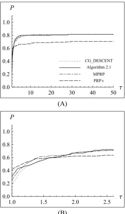
Figure 1 – Performance profiles relative to the CPU time.
Algorithm 2.1 is efficient for solving unconstrained optimal problems since CG_DESCENT has been regarded as one of the most efficient nonlinear conju-gate gradients. We also note that the performances of Algorithm 2.1, CG_DES-CENT and MPRP methods are much better than that of the PRP+ method.
6 Conclusion
CG_DESCENT Algorithm 2.1
MPRP PRP
10 20 30 40 50
0.0 0.2 0.4 0.6 0.8 1.0
P
(A)
1.0 1.5 2.0 2.5
0.0 0.2 0.4 0.6 0.8 1.0
P
(B)
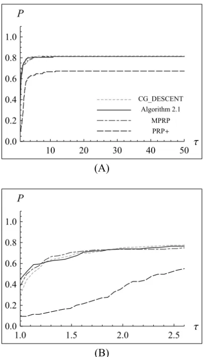
Figure 2 – Performance profiles relative to the number of iterations.
was efficient for solving the unconstrained problems in CUTEr library, and the numerical performance was similar to that of the wellknown CG_DESCENT and MPRP methods.
CG_DESCENT Algorithm 2.1
MPRP PRP
10 20 30 40 50
0.0 0.2 0.4 0.6 0.8 1.0 P
(A)
1.0 1.5 2.0 2.5
0.0 0.2 0.4 0.6 0.8 1.0 P
(B)
Figure 3 – Performance profiles relative to the number of function evaluated.
REFERENCES
[1] M.R. Hestenes and E.L. Stiefel, Methods of conjugate gradients for solving linear systems. J. Research Nat. Bur. Standards.,49(1952), 409–436.
[2] R. Fletcher and C. Reeves,Function minimization by conjugate gradients. Com-put. J.,7(1964), 149–154.
[3] B. Polak and G. Ribière, Note sur la convergence de méthodes de directions conjuguées. Rev. Française Informat. Recherche Opérationnelle,16(1969), 35– 43.
CG_DESCENT Algorithm 2.1
MPRP PRP
10 20 30 40 50
0.0 0.2 0.4 0.6 0.8 1.0
P
(A)
1.0 1.5 2.0 2.5
0.0 0.2 0.4 0.6 0.8 1.0
P
(B)
Figure 4 – Performance profiles relative to the number of gradient evaluated.
[5] R. Flectcher Practical Method of Optimization I: Unconstrained Optimization. John Wiley & Sons. New York (1987).
[6] Y. Liu and C. Storey, Efficient generalized conjugate gradient algorithms, Part 1: Theory. J. Optim. Theory Appl.,69(1991), 177–182.
[7] Y.H. Dai and Y. Yuan,A nonlinear conjugate gradient method with a strong global convergence property. SIAM J. Optim.,10(2000), 177–182.
[9] J.C. Gilbert and J. Nocedal,Global convergence properties of conjugate gradient methods for optimization. SIAM. J. Optim.,2(1992), 21–42.
[10] L. Zhang, W. Zhou and D. LiA descent modified Polak-Ribière-Polyak conjugate gradient method and its global convergence. IMA J. Numer. Anal.,26(2006), 629–640.
[11] G.H. Yu and L.T. Guan, Modified PRP Methods with sufficient desent property and their convergence properties. Acta Scientiarum Naturalium Universitatis Sunyatseni(Chinese),45(4) (2006), 11–14.
[12] Y.H. Dai, Conjugate Gradient Methods with Armijo-type Line Searches. Acta Mathematicae Applicatae Sinica (English Series),18(2002), 123–130.
[13] W.W. Hager and H. Zhang, A new conjugate gradient method with guaranteed descent and an efficient line search. SIAM J. Optim.,16(2005), 170-192. [14] M. Al-Baali, Descent property and global convergence of the Fletcher−Reeves
method with inexact line search. IMA J. Numer. Anal.,5(1985), 121–124. [15] Y.H. Dai and Y. Yuan, Convergence properties of the Fletcher-Reeves method.
IMA J. Numer. Anal.,16(2) (1996), 155–164.
[16] Y.H. Dai and Y. Yuan,Convergence Properties of the Conjugate Descent Method. Advances in Mathematics,25(6) (1996), 552–562.
[17] L. Zhang, New versions of the Hestenes-Stiefel nolinear conjugate gradient method based on the secant condition for optimization. Computational and Ap-plied Mathematics,28(2009), 111–133.
[18] D. Li and Fukushima, A modified BFGS method and its global convergence in nonconvex minimization. J. Comput. Appl. Math.,129(2001), 15–35.
[19] G. Zoutendijk,Nonlinear Programming, Computational Methods, in: Integer and Nonlinear Programming. J. Abadie (Ed.), North-Holland, Amsterdam (1970), 37–86.
[20] P. Wolfe, Convergence conditions for ascent methods. SIAM Rev., 11(1969), 226–235.
[21] P. Wolfe,Convergence conditions for ascent methods. II: Some corrections. SIAM Rev.,13(1969), 185–188.
[23] I. Bongartz, A.R. Conn, N.I.M. Gould and P.L. Toint, CUTE: Constrained and unconstrained testing environments. ACM Trans. Math. Software, 21 (1995), 123–160.
[24] E.D. Dolan and J.J. Moré,Benchmarking optimization software with performance profiles. Math. Program.,91(2002), 201–213.
[25] W.W. Hager and H. Zhang, A survey of nonlinear conjugate gradient methods. Pacific J. Optim.,2(2006), 35–58.
[26] D.F. Shanno,Conjugate gradient methods with inexact searchs. Math. Oper. Res.,
3(1978), 244–256.
[27] L. Zhang, W. Zhou and D. Li,Global convergence of a modified Fletcher-Reeves conjugate gradient method with Armijo-type line search. Numer. Math., 104
(2006), 561–572.