Searching for long-range dependence in real effective
exchange rate:
towards parity?
♦André M. Marques
Professor – Universidade Federal da Paraíba (UFPB)
Endereço: Campus I – Cidade Universitária, s/n, João Pessoa – Paraíba/PB – Brasil CEP: 58051-900 – E-mail: [email protected]
Fábio Pesavento
Coordenador do Núcleo de Economia Empresarial – (ESPM-Sul)
Endereço: Rua Guilherme Schell, 350 – Bairro Santo Antônio – Porto Alegre/RS – Brasil CEP: 90640-040 – E-mail: [email protected]
Recebido em 24 de abril de 2014. Aceito em 17 de outubro de 2014.
Abstract
After the widespread adoption of flexible exchange rate regime since 1973 the volatil-ity of the exchange rate has increased, as a consequence of greater trade openness and financial integration. As a result, it has become difficult to find evidence of the purchasing power parity hypothesis (PPP). This study investigates the possibility of a fall in the persistence of the real exchange rate as a consequence of the financial and com-mercial integration by employing monthly real effective exchange rate dataset provided by the International Monetary Fund (IMF). Beginning with an exploratory data analysis in the frequency domain, the fractional coefficient d was estimated employing the bias-reduced estimator on a sample of 20 countries over the period ranging from 1975 to 2011. As the main novelty, this study applies a bias-reduced log-periodogram regres-sion estimator instead of the traditional method proposed by GPH which eliminates the first and higher orders biases by a data-dependent plug-in method for selecting the number of frequencies to minimize asymptotic mean-squared error (MSE). Additionally, this study also estimates a moving window of fifteen years to observe the path of the fractional coefficient in each country. No evidence was found of a statistically significant change in the persistence of the real exchange rate.
Keywords
Purchasing power parity. Persistence. Fractional integration. Real exchange rate.
Resumo
Após a adoção generalizada do regime de câmbio flexível nos diversos países desde 1973, a volatilidade da taxa cambial aumentou, em contexto de maior abertura co-mercial e integração financeira. Tornou-se mais difícil encontrar evidências favoráveis
à hipótese da paridade do poder de compra. Este estudo analisa a possibilidade de queda na persistência da taxa de câmbio real como consequência da abertura comercial e integração financeira, com dados mensais de 20 países no período de 1975 a 2011. A partir de uma análise exploratória dos dados no domínio da frequência, o coeficien-te fracionário d foi obtido utilizando-se um estimador semiparamétrico com redução de viés em que um algoritmo dependente dos dados seleciona o número ótimo de frequências que minimiza o erro quadrático médio, diferente do estimador tradicional GPH. O estudo também utiliza uma janela móvel de 15 anos para identificar a evolução do coeficiente fracionário ao longo dos anos. Não há evidência de queda na persistência da taxa de câmbio real, nem indicações que corroborem a hipótese da paridade do poder de compra.
Palavras-Chave
Paridade do poder de compra. Persistência. Integração fracionária. Taxa de câmbio real.
Classiicação JEL F31. F41.
1. Introduction
One of the most controversial hypotheses in macroeconomics is the assertion that a homogeneous commodity sold in different countries must have the same selling price, in the different currencies, after the conversion by the exchange rate. Once taken the conversion, the differences observed in prices would be eliminated by arbitrage operations. In the aggregate, for all the different commodities and services, the corollary of the single price law is that the real exchan-ge rate should converexchan-ge to a constant in the long run, resulting in the hypothesis of purchasing power parity (PPP), which implies the stationarity of the real exchange rate. Although analyzing its relative version is of great importance, this work examines only its absolute version.1
The importance of this theoretical assumption is widely recognized in macroeconomics (Obstfeld and Rogoff, 1996: Chapter 4) with many known examples of its applications: choice of initial rates for a newly independent country, to forecast medium and long run for the real exchange rate, to make international comparisons of income,
since wages and prices are quoted in different units of measure.2
1 For a detailed exposition of the relative version of PPP hypothesis, see Sarno and Taylor (2002) and specially Rogoff (1996).
Regarding the study by Okimoto and Shimotsu (2010) which adopt a fractional approach to the issue, this study seeks to advance the following aspects: (1) selection of the most appropriate database to measure the long run persistence of exchange rate taking into account the weight of trade, (2) increased the data points and the number of countries, (3) use of a more efficient semiparametric estimator with reduced bias, (4) estimation of a fifteen-year mo-ving window, showing the path of persistence since 1980, along with the study by Okimoto and Shimotsu (2010) for comparison purpo-ses only. With these additions and modifications news results were found, similar to the ones found in the studies of Engel (2000) and Taylor and Taylor (2004).
In summary, the aim of this study is to investigate the hypothesis of purchasing power parity in a fractional perspective through the
semiparametric estimator introduced by Andrews and Guggenberger
(2003) (AGG) with reduced bias, in order to test the hypothesis of change in the persistence of the real effective exchange rate before and after the economic opening and financial liberalization of the 1990s. The use of a more appropriate basis for measuring competi-tiveness with more data points can provide more reliable evidence on the stationarity nature of the real exchange rate of the countries.
The central hypothesis suggested by Shimotsu and Okimoto (2010) is that the coefficient of persistence may have been reduced in most countries after the financial and trade integration since the 1990s by the action of the stabilizing factors mentioned below, which may have made the real exchange rate stationary towards purchasing power parity hypothesis. However, taking into account the weight of trade between economies, more countries and longer samples, the results do not corroborate the findings of previous studies and support the conclusions of Engel (2000) and Rogoff (1996).
For most of the countries in the sample there was an increase in the long run persistence of the real exchange rate. The null hypothesis of equal persistence before and after the institutional changes of the 1990s cannot be rejected at conventional levels of probability. We conclude that there is no statistically significant change in the persistence of the real exchange rate before and after the opening of trade and financial integration among economies. On the contrary, in many countries there is a positive trend in the persistence measure documented by the moving window of fifteen years.
The PPP hypothesis has been studied, in most cases, with the appli-cation of a wide variety of unit root tests. In these studies, it is observed that the specification of the model used, the time window and the database also vary. The rejection of the unit root hypothesis is interpreted as evidence in favor of PPP. In this perspective, with the data for the real exchange rate in a sample of twenty countries, Taylor (2002: 144) reports evidence favorable to the hypothesis of
purchasing power parity. Divino et al. (2009) and Kim and Lima
(2010) are other examples of recent studies using the approach of the unit root test in order to verify the PPP hypothesis.
Although some studies have found evidence favorable to this theo-retical assumption, Taylor and Taylor (2004: 143) conclude: “The flurry of empirical studies employing these types of tests (...) among major industrialized countries that emerged (...) were unanimous in their failure to reject the unit root hypothesis for major real ex-change rates – this was probably due to the low power of the tests”.
The low power of the unit root tests (especially ADF and PP) per-sisted in the literature, despite the fact that a variety of authors increased the sample size through simulations or added more obser-vations over time and also more countries in the database (Lothian and Taylor, 1997; Sarno and Taylor, 2002). Indeed, the addition of data for longer historical periods gave rise to the question of how to interpret these results, since they included so different exchange rate regimes or different historical periods from several decades (before 1973, for example).
nonstationary behavior of the exchange rate, consistent with the Balassa-Samuelson effect, by which developed countries have price levels significantly higher than developing countries because of the productive structure and the high share of services in the aggregate product, which complicates the equalization of prices internatio-nally postulated by purchasing power parity. In general, the results presented by Engel (2000) did not corroborate the PPP hypothesis. Similarly, Rogoff (1996) notes substantial price dispersion across countries, analyzing the data base by Summers and Heston (1991).
Besides the low power of unit root tests previously pointed out (Taylor and Taylor, 2004), another limitation of this approach is to investigate only the extreme cases, in which the process
{ }
X
t is con-sidered integrated of order d, denoted by Xt ~ ( )I d , where d can only assume the values zero or one: the series would have infinite persistence or no persistence. Because of these two limitations, in the same direction of the study by Okimoto and Shimotsu (2010), this study proposes the adoption of a fractional approach to find evi-dence on the hypothesis of purchasing power parity for a sample of twenty countries with monthly data from January 1975 to November 2011 provided by the International Monetary Fund (IMF, 2012).The fractional approach provides a more flexible alternative to the
above mentioned extreme cases, since the fractional coefficient d
can assume any real value in the interval
(
−
0.5;1
)
. The fractional ap-proach has been used to measure the long-range dependence (or long memory) in macroeconomic variables such as inflation, exchange rates, interest rates, unemployment, etc. In the Brazilian literature, Figueiredo and Marques (2009), after detecting evidence of long memory in two subsamples of the Brazilian inflation, fail to reject the hypothesis of inertial inflation and its persistence toinflation-ary or deflationinflation-ary shocks using the fractional coefficient d for the
Considering the international context, studies which measure the persistence of macroeconomic series suggest that it may have been significantly reduced after trade liberalization and the deepening of financial integration among economies. In particular, some authors argue that greater economic openness and capital account libera-lization would reduce the volatility of the output by favoring con-sumption smoothing, with beneficial effects on the growth of
cou-ntries (Kose et al., 2006). This wave of expansion of global finance
and trade interdependence has gradually expanded in industrialized countries during the 1970s and 1980s on the grounds of combating “financial repression”, and it expanded rapidly from the 1990s up to
the present time (Lane and Milesi-Ferretti, 2006; Kose et al., 2006).
Concurrently with the institutional changes mentioned, the early 1980s and 1990s also witnessed a spectacular expansion of parti-cipation of the Asian capital markets in the global capital markets.
Indeed, Arshanapalli et al. (1995) documented a substantial increase
in the interdependence between the capital markets of the United States, Japan, Hong Kong, Malaysia, Philippines, Singapore and Thailand after the 1987 crash. Additionally, Sensier and van Dijk (2004) found a decline of volatility in various economic series (em-ployment, consumption, wages and prices) in the United States from the mid-1980s, which may be contributing to the stabilization of the other economies, through greater interdependence. Still under this
perspective, Ahmed et al. (2004) reported a substantial decline in
U.S. output volatility in the period from 1984 to 2002 in the com-ponents of aggregate demand and consumer prices compared with the pre-1984 period, contributing to the stabilization of other eco-nomies. According to the authors, “the decline in output variability appears to be mirrored in all major demand-side and product-side components of GDP, as well as in the inflation rate and many other
macroeconomic and financial variables” (Ahmed et al., 2004, p. 824).
Despite the contribution of the above mentioned factors to the stabi-lization of the economies in general, the real exchange rate may have preserved its nonstationary character due to the substantial increase in volatility during the period of floating exchange rates (since 1973), with negative impacts on production and trade of various economies
(Rajan, et al. 2002). On this point, Rogoff (1996, p. 647) notes
that, for the period of one month, the volatility of the real exchan-ge rate is roughly the same volatility of the nominal exchanexchan-ge rate. According to Rogoff, “Price differential volatility is surprisingly large even when one confines attention to relatively homogenous classes of highly traded goods”.
Eichengreen et al. (1996) documented the contagion effect of
va-rious speculative attacks on the exchange rate in a sample of twenty industrial countries in the period between 1959 and 1993. The lar-gest commercial and financial integration among the economies may have contributed to strengthening the volatile nature of the exchan-ge rate. The authors conclude that currency crises increased by 0.08 the probability of speculative attacks, with adverse effects on the competition and trade in the country, regardless of macroeconomic fundamentals.
Having this set of factors that contribute to stabilizing the econo-mies and its possible impact on other countries with stronger trade and financial transactions, the question is whether these stabilizing influences are also being transmitted to the level of competitiveness of the countries in general, offsetting the increased volatility of the nominal exchange rate and its adverse effects on trade and pro-duction, supporting the hypothesis of purchasing power parity. The institutional changes implemented in several countries in the 1990s, such as the economic openness and greater financial integration, could have become the real stationary exchange rate, contributing to the fall in their persistence to shocks.
The paper is organized as follows. After the Introduction, section two describes the database and presents the methodology used in the study. Section three presents and discusses the results and in section four, the final comments are made.
2. Methodology
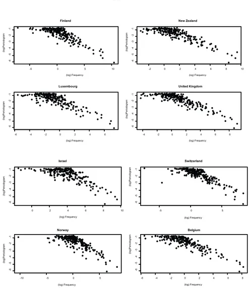
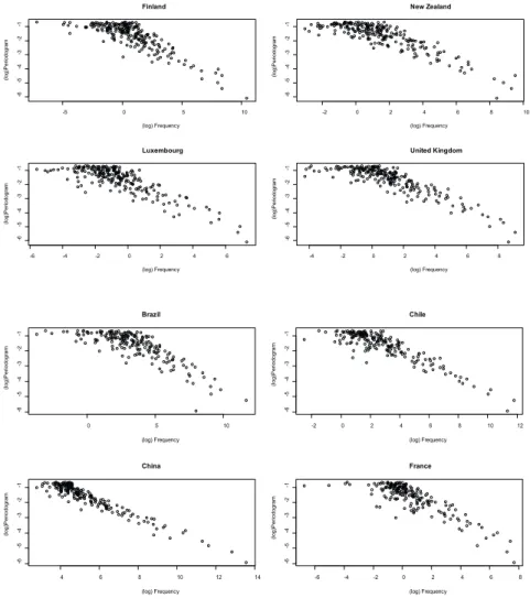
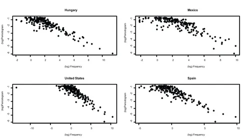
The steps adopted in this study were four. Initially, we seek evi-dence of fractional behavior with exploratory data analysis in the frequency domain, following the approach by Beran (1994), by ex-ploring scatter plots between frequency and periodogram, both in
logarithmic scale. Next, following the study by Baillie et al. (1996),
two complementary tests for stationarity/nonstationarity were com-bined in order to obtain evidence of fractional behavior, in which the rejection of the null hypothesis of both tests suggests that the series is neither I (1) nor I (0), but fractionally integrated. The basic
change in relation to the study by Baillie et al. (1996) is to apply
a more efficient test for time series with higher persistence
intro-duced by Elliott et al. (1996). A step further was made by applying
the unit root test introduced by Lee and Strazicich (2003) which considers the possibility of (two) occasional changes on level of the series.
Subsequently, we proceeded with the estimation of the fractional coefficient for full and partitioned samples before and after the in-tensification of financial integration. Finally, a moving window of fifteen years was estimated in order to observe the path of the long run persistence over time, to the extent that the economies beca-me more financially and combeca-mercially integrated. The evolution of the fractional coefficient is shown in the Appendix, in which the
horizontal line is attached to the unit (d=1), suggesting that the
persistence of the real exchange rate remains above the unit in most countries in the sample.
2.1. The dataset
this work covers the period from 1975:01 to 2011:11, generating an increase of about 5 years of data points with three added countries. The selection of the database to be used in the study takes into account the availability of monthly series for the post-1973 period
in the database of the International Monetary Fund (IMF, 2012).3
Now, we search for a measure of the exchange rate that may more accurately reflect the competitiveness between countries. Overall, most studies employ the real exchange rate without taking into ac-count the weight of trade between ac-countries. This choice of data has been criticized in the literature because the trade balance, through the availability of foreign money, tends to influence the level of the exchange rate.
There are well documented evidences that the trade balance strongly influences the behavior of the real exchange rate (Helmers, 1991; Joyce and Kamas, 2003; Okimoto and Shimotsu, 2010). Therefore, Cline and Williamson (2011: p. 2) note that “the relevant exchange rate concept is an effective rate, i.e., one which in foreign currencies are taken into account and weighted by their importance in the fo-reign trade of the country in question to form a single estimate of the exchange rate”. According to Cline and Williamson (2011), “The practice of measuring a currency’s value in terms of the currency of single trading partner and calling this ‘the exchange rate’ is quite wrong for any country with reasonably diversified trade”. For these reasons, the variable used in the study was the real effective exchan-ge rate based on consumer price index for each individual country, extracted from the CD-Rom of the International Monetary Fund (IMF, 2012).
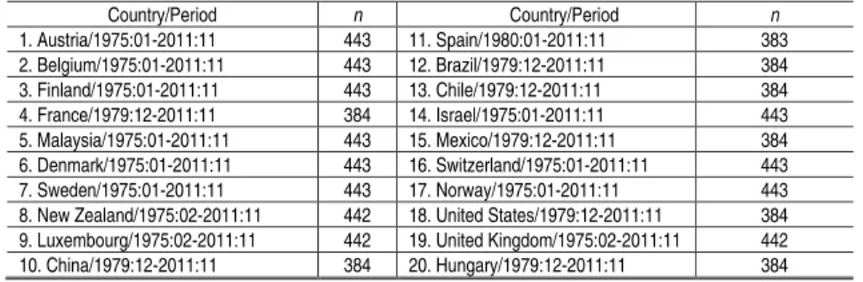
Nevertheless, since for some specific countries and periods there were no observations available, the Table 1 below presents in de-tails the country and also the period in which data were available,
with the respective sample size (n) for the estimations. The choice
of the time period can be justified historically. Indeed, like Taylor and Taylor (2004: 141) observes: “in 1971, President Nixon ended the convertibility of the U.S. dollar relative to gold. After failed
3 The complete sample of countries at IMF’s CD-ROM was thirty. However, for Canada,
attempts to restore a version of the Bretton Woods agreement, the major currencies of the world began floating against each other in March 1973”.
For some countries, data were available before 1975, however, this year was chosen as the initial period because it reflects the historical widespread adoption of generalized floating exchange rate regime for the sample countries.
Table 1 - Sample of countries – several periods
Country/Period n Country/Period n
1. Austria/1975:01-2011:11 443 11. Spain/1980:01-2011:11 383
2. Belgium/1975:01-2011:11 443 12. Brazil/1979:12-2011:11 384
3. Finland/1975:01-2011:11 443 13. Chile/1979:12-2011:11 384
4. France/1979:12-2011:11 384 14. Israel/1975:01-2011:11 443
5. Malaysia/1975:01-2011:11 443 15. Mexico/1979:12-2011:11 384
6. Denmark/1975:01-2011:11 443 16. Switzerland/1975:01-2011:11 443
7. Sweden/1975:01-2011:11 443 17. Norway/1975:01-2011:11 443
8. New Zealand/1975:02-2011:11 442 18. United States/1979:12-2011:11 384 9. Luxembourg/1975:02-2011:11 442 19. United Kingdom/1975:02-2011:11 442
10. China/1979:12-2011:11 384 20. Hungary/1979:12-2011:11 384
Source: Authors’ elaboration based on data extracted from the CD-Rom of IMF (2012).
2.2 Exploratory data analysis: periodogram and frequency
The long memory coefficient d measures the persistence of a
va-riable in the long run and it is generally identified from the slow hyperbolic decay of the autocorrelations at high lags of a time se-ries. In the frequency domain, however, the analysis of the periodo-gram along with the frequencies can suggest the slow (hyperbolic) decay of autocorrelations. In this case, the long-range dependence is suggested from the occurrence of inverse correlation (on a loga-rithmic scale) between frequency and periodogram, in which the absence of long memory is identified by random scattering around a constant situated near the origin of the periodogram.
was constructed from the ordered pairs of periodogram
I
j( )
⋅
andfrequencies (
λ
j) defined in the expression (5) below.2.3. Semiparametric estimator by Andrews-Guggenberger (2003) (AGG)
Since the contribution by Robinson (1995) the semiparametric esti-mation of fractional coefficient d has been an active area of research. In the frequency domain, two approaches have been intensively stu-died in the literature: the regression of the logarithm of the periodo-gram (GPH, Geweke and Porter-Hudak, 1983) and the local Whittle estimator (LW, Künsch, 1987). The GPH estimator has been widely criticized for its strong bias in finite samples (Agiakloglou, Wohar and Newbold, 1993).
More recently, Andrews and Guggenberger (2003) introduced a new estimator with similar properties to the traditional GPH, but with two very desirable features: with elimination of bias for small and large samples and higher speed of convergence to zero of the mean -squared error (MSE) relative to the GPH and Whittle estimators. Indeed, this study applies a bias-reduced log-periodogram regression estimator instead of the traditional method proposed by Geweke and Porter-Hudak (1983) (GPH). The main advantage of this alter-native method is to eliminate the first and higher orders biases of the GPH estimator. It employs assumptions on the spectrum only in the zero frequency neighborhood with a data-dependent plug-in method for selecting the number of frequencies in order to minimize asymptotic mean-squared error (MSE).
Okimoto and Shimotsu (2010) employ a variation of the local Whittle estimator, which does not require the use of pre-filter (dif-ferentiation) in series in order to estimate fractional coefficient. There are still no comparative studies measuring the efficiency of these estimators.
Consider
− ∈
2 1 , 2 1
d the order of integration of a fractional
pro-cess. The process Xtintegrated of order d is defined by:
where
µ
is the mean, Bis the lag operator and{ }
ut t∈Z has zeromean and constant variance. Where,
2 30
( 1) ( 1)( 2) ( )
1 1 ...
2! 3! ( ) ( 1)
p d
p
d d B d d d B p d B
B dB d p
(2)
in which
Γ ⋅
( )
is the gamma function. It is said that the processt
X has long memory if
∈ 2 1 , 0
d , short memory if
d
=
0
, and itis considered antipersistent if
−
∈ ,0
2 1
d , it will be a long memory
process (nonstationary), with infinite variance, but reversible to the
average if
∈ ,1
2 1
d . In the case of d greater than the unit, the
pro-cess exhibits infinite persistence and is nonstationary.
The semiparametric estimator proposed by Andrews-Guggenberger (2003) is the same one introduced by GPH, except for the inclusion of frequencies in the power 2k, for k=1, 2,...,r for some positive
integer r as additional covariates of pseudoregression introduced by
the GPH.
Consider the semiparametric model for the stationary Gaussian pro-cessXt: t=1, 2,...,n. The spectral density for the series is given by
2
( ) d ( )
f
g
(3)
where d is the coefficient of long memory, in which
g
( )
⋅
is an even function which is continuous at zero with0
<
g
( )
0
< ∞
. GPH pro-posed a reparametrization of equation (3), wherein:
2 *
1 exp
df
i
f
(4)
in which
f
*( )
⋅
satisfies the same conditions of g(⋅), and for the firstordered m frequencies of the periodogram Ij, defined by:
21
1
exp , 1, 2,..., . 2
n
j t j
t
I X it j m
n
Where j 2 j n
π
λ
= , m is a positive integer lower than n. The GPHestimator is given by 1
2
− multiplied by the least squares
estima-tor of the slope coefficient in a regression of {logIj: j=1,..., }m on
a constant and the regressor variable
X
t=
log 1 exp
−
( )
−
i
λ
j . TheGPH fractional coefficient is defined by,
1
2
1
0.5 log
ˆ
m
j j
i
GPH m
j i
X X I
d
X X
(6)
where
1
1
. m
j i
X X
m =
=
∑
According to the specification by Robinson
(1995), AGG leave the term -0.5 of the equation (6) and
X
j issubstituted byXj = −2 log
λ
j. And in the periodogrampseudore-gression
λ λ
2j,
4j,...,
λ
2jr covariates are added, resulting in drwith re-duced estimator bias for small and large samples with significantly better performance than the GPH estimator. In practice, the authors suggest lower values for r(r=1, 2). In case ofr
=
0
, dr isasymp-totically equivalent to traditionaldGPH . Throughout this study it is
assumed thatr=1, given the lower standard error of the estimated
coefficients.
The importance of choosing the AGG estimator is justified by the following reasons. First, in the simulations to measure the efficiency and bias of the estimator, AGG estimator showed better perfor-mance compared with other semiparametric estimators (Whittle and
GPH). Second, an integrated process of order d, with
d
∈ −
(
0.5,1
)
,can accommodate the slow hyperbolic decay of both autocorrelations
and impulse response functions that are inconsistent with I(1) or
) 0 (
I . The long run dynamics of this process is governed solely by
fractional coefficient d, which is a measure of persistence to shocks.
Third, as shown by Hosking (1981) and Kumar and Okimoto (2007),
the estimated fractional coefficient d as a measure of long run
per-sistence does not require a specific formulation about short run
moving average – MA coefficients).4 In other words, no assumptions are made about the exact structure of the data generating process in the short run. Indeed, these authors show that it is possible to reach quite diverging conclusions by measuring short run persistence with measures based on autoregressive coefficient (like largest autoregres-sive root – LARR and the sum of autoregresautoregres-sive coefficients – SARC
measures) and the long run persistence with fractional coefficient d,
since these two different approaches render different information and determine different behaviors of the impulse response function of the series.5
Additionally, in a semiparametric approach, the estimation of AR and MA components can impose important constraints on the frac-tional coefficient in small samples. About this, Sowell notes that: “The result is that the fit of the long-run behavior of the series may be sacrificed to obtain a better fit of the short-run behavior” (Sowell, 1992, p. 279).
2.4. Partitioning of the sample
Initially, we analyzed the literature which discusses the financial integration and economic liberalization aimed at detecting a time change considered reasonable to separate the sample into two parts. The hypothesis is that the acceleration of financial and commercial integration changed the long run persistence of real exchange rate. According with Lane and Milesi-Ferreti (2003, p. 86; 2006, p. 15), the scale of international financial integration can be measured by
it it
it
it
FA
FL
IFIGDP
GDP
(7)
where
IFIGDP
it is the calculated measure of financial integration forcountry i at time t,
FA
it(
FL
it)
denotes the stock of external assets(liabilities) and
GDP
it is the per capita Gross Domestic Product.This de facto measure of financial integration was calculated for
71 countries including developed and developing economies for the
4 For a detailed approach of LARR and SARC measures of short run persistence, see Pivetta and Reis (2007).
period from 1970 to 2004 by those authors. By analyzing the path of this measure we can conclude that its acceleration take place around 1990-5 in developed and developing economies (see Lane and Milesi-Ferreti, 2006, p. 65, Figure 3).
In this study, there was no attempt to identify the exact date that would indicate a structural change in the path of index of financial integration between economies measured by (7), or whether these changes are abrupt or smooth. An additional study would be ne-cessary to answer that question. Therefore, the hypothesis testing performed in this study can be considered conservative because it is statistically significant only if the change in the fractional coefficient is substantially big. This results interpretation is complemented by the very useful estimation of the fractional coefficient from a mo-ving window of fifteen years for the sample of 20 countries. With this procedure we can visualize the history of the long run persisten-ce in each country individually and the effects of theses institutional reforms on it along the decades. This procedure can offer valuable
information about the stability of coefficient d along the years and
has been used in a number of representative works on time series
(see references in Banerjee et al., 1992; Kumar and Okimoto, 2007).
As noted before, the measure of financial integration presented by Lane and Milesi-Ferretti (2006) provides strong evidence that the
acceleration of financial integration took place in the mid-1990s,6
and then the sample was divided into two periods: 1975-1994 and 1995-2011. Additionally, Santos-Paulino (2002, Tab.1) also suggest, on average, the same year to the trade openness of most countries of the sample. This criterion to partition of sample is absent in the study by Okimoto and Shimotsu (2010), then we expect that our results to be more correlated with institutional changes bypassed by these countries.
Also in relation to those authors, in this paper the absence of a test to indicate the presence of long memory in the series was overcome by carrying out tests of hypotheses for the combined stationarity/ nonstationarity, complemented by descriptive analysis in frequency domain. In general, it is trivial to use only the estimation of the au-tocorrelation function at high lags as evidence of long memory and the significance test of the fractional coefficient (see Kumar and Okimoto, 2007; Figueiredo and Marques, 2009).
Following an examination of the literature and the separation of the sample into two parts based on the study mentioned above, we
proceeded with the estimation of the fractional coefficient d for
each period separately. The evolution of the fractional coefficient, subject to major economic events such as the financial crises of the 1990s, may have changed the data distribution, as well as the mean and variance of the process. So, the study wants to compare two populations without assuming that their distributions are normal and homoscedastic. For this end, nonparametric Wilcoxon test for related samples was applied.
Once estimated the fractional coefficient for each historical subpe-riod, the hypothesis to be tested is the equality of the persistence of the two periods (d1 =d2) against the alternative hypothesis of a fall in the persistence of real exchange rate
(
d
1>
d
2)
due to the reasons explained in the Introduction.3. Results and discussion
In this section, the results are reported for the four stages of the study: exploratory data analysis using the periodogram and frequen-cy of the real effective exchange rate data; tests for stationarity/ nonstationarity with different null hypotheses; estimation of per-sistence for the full sample and partitioned one; testing for change in persistence; analysis of the temporal evolution of the measure of persistence to a 15-year moving window.
3.1 Evidence of fractional integration
the origin. The further procedure for detecting signs of long memory
is the same one adopted by Baillie et al. (1996), which consisted
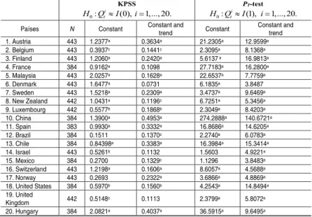
of using two joint tests to verify that the data were not consistent with a process I (1) neither with process I (0). The basic idea is that the rejection of both null hypotheses of the tests (KPSS-test and
PT-test) provides evidence of fractional behavior. As reported by
Taylor and Taylor (2004), the traditional ADF and PP tests have low power against alternatives of high persistence. For this reason, the Phillips and Perron (1988) test, used in conjunction with the KPSS test by Baillie et al. (1996), was replaced by the PT-test, which null
hypothesis is a unit root. This test is considered efficient for high persistent series and showed better performance in the simulations
by Elliot et al. (1996) compared with ADF and PP tests. The KPSS
test has stationarity as the null hypothesis. The results of both tests are shown in table 2 below. The results shown in Table 2 are consis-tent with the information gathered in the scatter plot shown in the Appendix, in which the autocorrelations are not summable.
Table 2 - Testing for the order of integration of the real effective exchange rate - results
KPSS
0: (0), 1,..., 20. i
t
H Q I i
PT-test
0: (1), 1,..., 20. i
t
H Q I i
Países N Constant Constant and trend Constant Constant and trend
1. Austria 443 1.2377a 0.3634a 21.2305a 12.9599a
2. Belgium 443 0.3937c 0.1441c 2.3095a 8.1368a
3. Finland 443 1.2060a 0.2420a 5.6137 a 16.9813a
4. France 384 0.9162a 0.1098 27.7183a 16.2800a
5. Malaysia 443 2.0257a 0.1628a 22.6537a 7.7759a
6. Denmark 443 1.6477a 0.0731 6.1835a 3.8487 7. Sweden 443 1.5218a 0.2309a 3.4737a 9.6469a
8. New Zealand 442 1.0431a 0.1196c 6.7251a 5.3456a
9. Luxembourg 442 0.5577b 0.1868b 2.3049a 8.4203a
10. China 384 1.3900a 0.4953a 274.2888a 140.6721a
11. Spain 383 0.9930a 0.3332a 16.8686a 14.6205a
12. Brazil 384 0.1511 0.1370c 2.2740a 6.0783a
13. Chile 384 0.84398a 0.3383a 16.3984a 15.3414a
14. Israel 443 0.5261b 0.1132 1.5603 4.9221a
15. Mexico 384 0.2700 0.1329c 1.1296 3.8483a
16. Switzerland 443 1.2198a 0.1606a 8.6057a 4.5688a
17. Norway 443 0.2693 0.2322a 3.6866a 4.8869a
18. United States 384 0.5970b 0.1560b 4.2543a 14.8494a
19. United
Kingdom 442 0.5148c 0.1113 2.3799a 5.8072a 20. Hungary 384 2.0821a 0.4037a 36.5915a 9.6495a
Note: critical values for PT-test: only constant = (1%, 5%, 10%) 1.9900; 3.2600; 4.4800. PT-test: with constant and trend = (1%, 5%, 10%) 3.9600; 5.6200; 6.8900. Critical values for KPSS test: only constant = (10%, 5%, 1%) 0.3470; 0.4630; 0.7390. KPSS test with constant and trend = (10%, 5%, 1%) 0.1190; 0.1460; 0.2160. Critical values for PT-test extracted from Elliot et. al.
(1996, Table 1, p. 825). (a) Significant at 1% probability; (b) significant at 5% probability; (c) significant at 10% probability. The number of additional lags (k) was obtained by the expression:
k = integer {4(T/100)¼} following Kwiatkowski et. al. (1992).
At 5% and 10% probability, these results suggest the occurrence of fractional integration in all countries of the sample, i.e., the series, in general, cannot be considered either I (1) or I (0), since in most cases there is strong evidence against the null hypothesis in both tests. In particular, among the twenty countries, only in the case of Belgium, Brazil, Mexico and United Kingdom the stationarity (KPSS) null hypothesis is rejected at 10% probability. In all other cases, the rejection occurs at 1% and 5% probability. In all cases, the
results of the PT-test suggest rejection of the unit root hypothesis
at 1% probability. These two tests above (KPSS and PT-test) do not
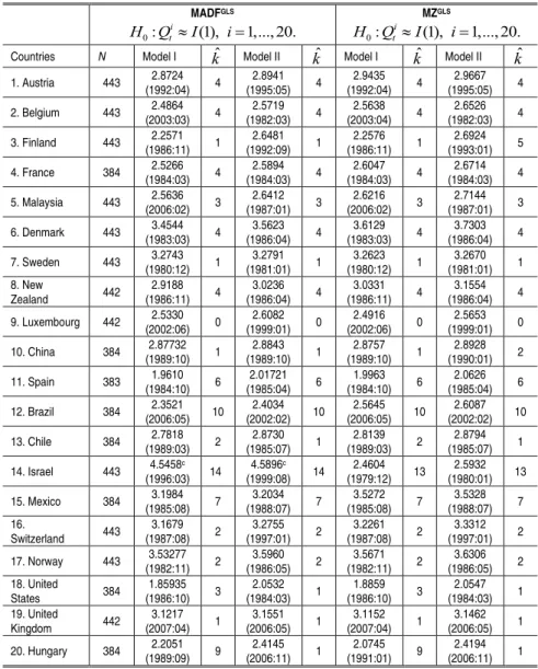
take into account possible structural changes in trend function of the series. Then, to test for persistence, we apply two additional unit root tests by considering one and two possible structural changes in the trend function at unknown time. First, we apply unit root test introduced by Perron and Rodríguez (2003) based on GLS
de-trending approach introduced by Elliot et al. (1996). The Table 3
presents the results for M and ADF tests choosing the date which minimizing the test statistics. 7
7
Table 3 - Testing for the order of integration of the real effective exchange rate - results
MADFGLS
0: (1), 1,..., 20.
i t
H Q I i
MZGLS
0: (1), 1,..., 20.
i t
H Q I i
Countries N Model I kˆ Model II kˆ Model I kˆ Model II kˆ
1. Austria 443 (1992:04) 2.8724 4 (1995:05) 2.8941 4 (1992:04) 2.9435 4 (1995:05) 2.9667 4
2. Belgium 443 2.4864 (2003:03) 4
2.5719 (1982:03) 4
2.5638 (2003:04) 4
2.6526 (1982:03) 4
3. Finland 443 2.2571 (1986:11) 1
2.6481 (1992:09) 1
2.2576 (1986:11) 1
2.6924 (1993:01) 5
4. France 384 (1984:03) 2.5266 4 (1984:03) 2.5894 4 (1984:03) 2.6047 4 (1984:03) 2.6714 4
5. Malaysia 443 2.5636 (2006:02) 3
2.6412 (1987:01) 3
2.6216 (2006:02) 3
2.7144 (1987:01) 3
6. Denmark 443 3.4544 (1983:03) 4
3.5623 (1986:04) 4
3.6129 (1983:03) 4
3.7303 (1986:04) 4
7. Sweden 443 (1980:12) 3.2743 1 (1981:01) 3.2791 1 (1980:12) 3.2623 1 (1981:01) 3.2670 1
8. New
Zealand 442
2.9188 (1986:11) 4
3.0236 (1986:04) 4
3.0331 (1986:11) 4
3.1554 (1986:04) 4
9. Luxembourg 442 2.5330 (2002:06) 0
2.6082 (1999:01) 0
2.4916 (2002:06) 0
2.5653 (1999:01) 0
10. China 384 (1989:10) 2.87732 1 (1989:10) 2.8843 1 (1989:10) 2.8757 1 (1990:01) 2.8928 2
11. Spain 383 1.9610 (1984:10) 6
2.01721 (1985:04) 6
1.9963 (1984:10) 6
2.0626 (1985:04) 6
12. Brazil 384 2.3521 (2006:05) 10
2.4034 (2002:02) 10
2.5645 (2006:05) 10
2.6087 (2002:02) 10
13. Chile 384 (1989:03) 2.7818 2 (1985:07) 2.8730 1 (1989:03) 2.8139 2 (1985:07) 2.8794 1
14. Israel 443 4.5458c (1996:03) 14
4.5896c
(1999:08) 14
2.4604 (1979:12) 13
2.5932 (1980:01) 13
15. Mexico 384 3.1984 (1985:08) 7
3.2034 (1988:07) 7
3.5272 (1985:08) 7
3.5328 (1988:07) 7 16.
Switzerland 443
3.1679 (1987:08) 2
3.2755 (1997:01) 2
3.2261 (1987:08) 2
3.3312 (1997:01) 2
17. Norway 443 3.53277 (1982:11) 2
3.5960 (1986:05) 2
3.5671 (1982:11) 2
3.6306 (1986:05) 2 18. United
States 384
1.85935 (1986:10) 3
2.0532 (1984:03) 1
1.8859 (1986:10) 3
2.0547 (1984:03) 1 19. United
Kingdom 442
3.1217 (2007:04) 1
3.1551 (2006:05) 1
3.1152 (2007:04) 1
3.1462 (2006:05) 1
20. Hungary 384 2.2051 (1989:09) 9
2.4145 (2006:11) 1
2.0745 (1991:01) 9
2.4194 (2006:11) 1
Note: The estimated dates are between brackets. Critical values for MADFGLS: Model I = (1%,
5%, 10%) -5.89; -4.61; -4.17 and Model II = (1%, 5%, 10%) -6.41; -4.98; -4.41. Critical values for MZGLS: Model I = (10%, 5%, 1%) -4.89; -4.19; -3.88 and Model II = (10%, 5%, 1%) -4.99;
-4.31; -4.07. All critical values were extracted from Perron and Rodríguez (2003, p. 10, Tab. 1). (a) Significant at 1% probability; (b) significant at 5% probability; (c) significant at 10% probabi-lity. The number of additional lags (k) was obtained by the sequential t-test at 10% of significance because in case of applying MADFGLS by minimizing the test statistic and for all data-dependent
methods, according to the authors “the power is high for all methods to choose k” (Perron and Rodríguez, 2003, p. 13). See Perron and Rodríguez (2003, p. 12-13) for details of the procedure, results of simulations and comparisons between three different criteria.
The main conclusion to extract from above results presented in
Ta-ble 3, in marked contrast with the results of PT-test, and in line
with the KPSS test results above (Table 2), is that we are unable to reject unit root test in all cases, except Israel at 10% probability. As mentioned before, a step further was made by applying the Lee and Strazicich (2003) unit root test by allowing for two occasional structural changes, by considering the questions raised by Perron (1989) influential work on unit root tests. Perron (1989) argues that by ignoring structural changes in the level and/or trend, traditional unit root tests may produce misleading results.
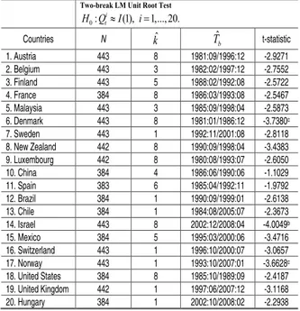
Then, we apply more recent two-break minimum LM unit root test introduced by Lee and Strazicich (2003) in an augmented version to correct for serial correlation. Following Perron (1989), Zivot and Andrews (1992), and Lee and Strazicich (2003), we assume the “crash” model (model A) for all series of real effective exchange
rates.8 In the same fashion of the authors, by starting from a
maxi-mum of k = 8 lagged terms, the procedure looks for significance of
the last augmented term, fixed in 0.10. After determining the opti-mal at each combination of two breaks, the breaks are determined
where the LM t-test statistic is at a minimum. The results are shown
in the Table 4 below.
The results exposed in Table 4 suggest that we are unable to reject null of nonstationarity in almost cases, except Denmark, Israel and Norway at 5% and 10% probability. Important to note that these results are in accordance with the rejection of null of KPSS test, which point out nonstationarity for almost countries of the sample.
The general conclusion which we may extract from the results ex-posed in Tables 2, 3, and 4 below is that there are close concordance
between KPSS, MADFGLS and minimum LM unit root tests: for this
sample of countries, even by allowing for multiple structural changes in the trend function, the real effective exchange rates exhibits high persistence in an environment of higher financial and commercial integration with flexible exchange rates.
8
Table 4 - Testing for the order of integration of the real effective exchange rate - results
Two-break LM Unit Root Test
0: (1), 1,..., 20.
i t
H QI i
Countries N kˆ Tˆb t-statistic 1. Austria 443 8 1981:09/1996:12 -2.9271 2. Belgium 443 3 1982:02/1997:12 -2.7552 3. Finland 443 5 1988:02/1992:08 -2.5722 4. France 384 8 1986:03/1993:08 -2.5467 5. Malaysia 443 3 1985:09/1998:04 -2.5873 6. Denmark 443 8 1981:01/1986:12 -3.7380c
7. Sweden 443 1 1992:11/2001:08 -2.8118 8. New Zealand 442 8 1990:09/1998:04 -3.4383 9. Luxembourg 442 8 1980:08/1993:07 -2.6050 10. China 384 4 1986:06/1990:06 -1.1029 11. Spain 383 6 1985:04/1992:11 -1.9792 12. Brazil 384 1 1990:09/1999:01 -2.6138 13. Chile 384 1 1984:08/2005:07 -2.3673 14. Israel 443 8 2002:12/2008:04 -4.0049b
15. Mexico 384 5 1995:03/2000:06 -3.4716 16. Switzerland 443 1 1996:10/2000:07 -3.0657 17. Norway 443 1 1993:10/2007:01 -3.6628c
18. United States 384 8 1985:10/1989:09 -2.4187 19. United Kingdom 442 1 1997:06/2007:12 -3.1168 20. Hungary 384 1 2002:10/2008:02 -2.2938
Note: Critical values extracted from Lee and Strazicich (2003, table 2): -4.545 (1%); -3.842 (5%); -3.504 (10%); (a) significant at 1% probability; (b) significant at 5% probability; (c) signi-ficant at 10% probability.
Source: Authors’ calculations from the dataset provided by IMF (2012).
This conclusion contradicts with the approach and conclusions of
Baillie et al. (1996) which applied two complementary unit root
tests to detect fractional behavior probably because of they do not take into account occasional changes in the level and/or trend of the series. This observation casts more cautions on the analysis of unit root test to infer fractional behavior and more attention has to be paid on periodogram and frequency analysis, since it is the main indication for fractional behavior suggested by Beran (1994). With the additional information obtained by the scatter diagrams in the Appendix (periodogram and frequency) along with the significance
of fractional coefficient d, the conclusion reached in this study is
By the reasons exposed in the Introduction we move away from unit root tests and their extreme conclusions, where the series can be vie-wed only integrated of order 1 or 0 and adopt a more flexible alterna-tive by estimating the fractional coefficient d, which is not a integer and is the only measure for long run persistence of series, since it not depend upon autoregressive coefficient of unit root tests analyzed be-fore, which measure only its short run memory (short run persistence).
3.2. Results for full/partitioned sample. Test for change in persistence
The results of Table 5 below were obtained by the AGG estimator by applying the filter of the first difference. As the number of differenti-ated process I(d) isI(d−1), then the fractional coefficient was ini-tially estimated for the first difference of the real effective exchange rate and, in the end, the fractional coefficient dr is obtained by
sum-ming up the unit with the coefficient d estimated in first difference.
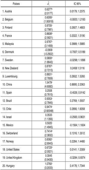
Then a confidence interval of 0.95 probability using the normal distri-bution was calculated. The results reported above, taking into account the confidence interval of 0.95, strongly suggest the nonstationary behavior of the real exchange rate in almost all sample countries ex-cept Denmark, Israel and United Kingdom, since the hypothesis of unit root cannot be rejected at 0.05 probability in the remaining cases.
December 2011. Summing up, we have 20 countries with monthly data from 1975 to November 2011. It is important to note, however, that trade and financial liberalization has intensified since the 1990s, as indicated by the studies by Lane and Milesi-Ferretti (2003,
2006), Santos-Paulino (2002) and Kose et al. (2006) applying the
measure of financial integration between countries.
Table 5 - Estimates for the full sample – ARFIMA
(
0,dr, 0)
Países dˆr IC 95%
1. Austria 0.6277b
(2.0177) 0.0179; 1.2375
2. Belgium 0.6095b
(1.95918) -0.0003; 1.2193
3. Finland (2.7981) 0.8705c 0.2607; 1.4803
4. France 0.8606b
(2.5621) 0.2022; 1.5190
5. Malaysia (3.1459) 0.9787c 0.3689; 1.5885
6. Denmark -0.0909
(-0.2922) -0.7007; 0.5189
7. Sweden 0.5800a
(1.8643) -0.0298; 1.1898
8. New Zealand (2.7213) 0.8787c 0.2458 1.5116
9. Luxembourg 0.8931c
(2.7659) 0.2602; 1.5260
10. China (4.6082) 1.5479c 0.8895; 2.2063
11. Spain 0.2558
(0.7615) -0.4026; 0.9142
12. Brazil 0.9353c
(2.7845) 0.2769; 1.5937
13. Chile (2.82048) 0.9474c 0.2890; 1.6058
14. Israel 0.3533
(1.1356) -0.2565; 0.9631
15. Mexico (1.4945) 0.5020 -0.1564; 1.1604
16. Switzerland 0.7414b
(2.3832) 0.1316; 1.3512
17. Norway 0.8382c
(2.6943) 0.2284; 1.4480
18. United States 0.6725b
(2.0021) 0.0141; 1.3309
19. United Kingdom 0.3045
(0.9430) -0.3284; 0.9374
20. Hungary (3.2033) 1.0760c 0.4176; 1.7344
Note: the sample period of each country is the same as described in table 1. T statistics calcula-ted between brackets. Critical values (probability): 1.66 (0.10); 1.96 (0.05); 2.58 (0.001). (a) Significant at 1% probability; (b) significant at 5% probability; (c) significant at 10% probability.
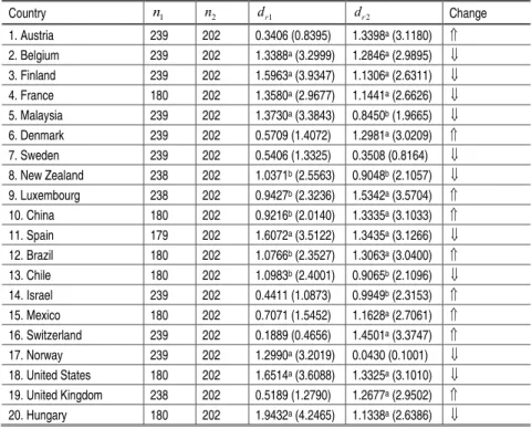
Analyzing the results shown in Table 6 below, two important con-clusions can be drawn.
First off all, some countries like Malaysia, Sweden and Norway have experienced a remarkable decrease in long run persistence. And on the other hand, some countries (Austria, Mexico, Switzerland, Luxembourg, United Kingdom and Denmark) showed a substantial increase in persistence, becoming more unstable after the institutio-nal reforms of that period.
Table 6 - Estimates for the partitioned sample - 1975:01-1994:12; 1995:01-2011:11
Country n1 n2 dr1 dr2 Change
1. Austria 239 202 0.3406 (0.8395) 1.3398a (3.1180)
2. Belgium 239 202 1.3388a (3.2999) 1.2846a (2.9895)
3. Finland 239 202 1.5963a (3.9347) 1.1306a (2.6311)
4. France 180 202 1.3580a (2.9677) 1.1441a (2.6626)
5. Malaysia 239 202 1.3730a (3.3843) 0.8450b (1.9665)
6. Denmark 239 202 0.5709 (1.4072) 1.2981a (3.0209)
7. Sweden 239 202 0.5406 (1.3325) 0.3508 (0.8164)
8. New Zealand 238 202 1.0371b (2.5563) 0.9048b (2.1057)
9. Luxembourg 238 202 0.9427b (2.3236) 1.5342a (3.5704)
10. China 180 202 0.9216b (2.0140) 1.3335a (3.1033)
11. Spain 179 202 1.6072a (3.5122) 1.3435a (3.1266)
12. Brazil 180 202 1.0766b (2.3527) 1.3063a (3.0400)
13. Chile 180 202 1.0983b (2.4001) 0.9065b (2.1096)
14. Israel 239 202 0.4411 (1.0873) 0.9949b (2.3153)
15. Mexico 180 202 0.7071 (1.5452) 1.1628a (2.7061)
16. Switzerland 239 202 0.1889 (0.4656) 1.4501a (3.3747)
17. Norway 239 202 1.2990a (3.2019) 0.0430 (0.1001)
18. United States 180 202 1.6514a (3.6088) 1.3325a (3.1010)
19. United Kingdom 238 202 0.5189 (1.2790) 1.2677a (2.9502)
20. Hungary 180 202 1.9432a (4.2465) 1.1338a (2.6386)
Note: t statistics between brackets. Critical values (probability): 1.66 (0.10); 1.96 (0.05); 2.58 (0.001). (a), (b), (c) statistically significant at 0.01; 0.05; and 0.10 of probability, respectively.
Importantly, these last two countries (United Kingdom and Denmark) had low persistence before the mid-1990s. Excepting the case of Malaysia, Sweden, Chile and Israel, there is no evidence of stationarity for the real effective exchange rate in any of the other countries in the sample, since the fractional coefficient is not located below the unity. Furthermore, in nine cases there was a substantial increase in the persistence of the real exchange rate and not a de-crease, as previously pointed out by some authors (see, for example, Okimoto and Shimotsu, 2010). In other cases, the observed decrease in persistence was not enough to make the exchange rate stationary, which coefficient remained substantially above unity after the ins-titutional reforms of the mid-1990s.
Indeed, this result is consistent with Lee and Strazicich (2003) test for high persistence with corroborate with the conclusion that trade and financial integration may help to explain the advent of more instable economies in the last decades when we consider the long run persistence of its real exchange rate. The increased volatility of exchange rate may have to contribute to cross and maintain persis-tence higher than unity (Rogoff, 1996; Engel, 2000). Another aspect that can be considered a potential candidate to explain these beha-viors is the ‘edge’ between international prices and the existence of non-tariff barriers to trade. All these aspects may have contributed to high long run persistence and more instable competitiveness of countries. The last issue to be addressed from the aforementioned results is whether this change in the persistence of real exchange rate can be systematically generalized to be considered for a large number of countries, as the Table would suggest, or whether no sig-nificant change occurred in persistence even with the institutional changes introduced in the mid-1990s.
The last column of Table 6 point out the directions of variation in
fractional coefficient d, but these observations does not permit to
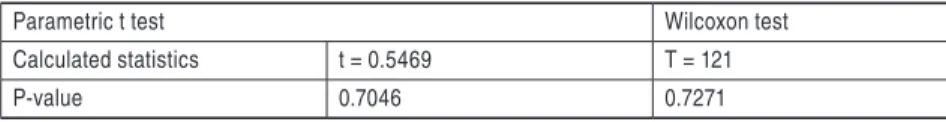
infer general and systematic conclusions. Visually it is difficult to know the final balance from the last column of Table 6, if there was an increase or systematic decline in the persistence of the exchange rate on aggregate countries. Therefore, this question can be answe-red with a test for change in persistence, in which the hypothesis of maintenance of persistence is tested against the hypothesis of decrease in persistence.
The Wilcoxon test requires assigning scores for each fractional diffe-rence between the two coefficients obtained under different condi-tions (before and after 1995). These differences are ranked and the sum of the positions results in a statistical T, which value depends on
the size of paired samples (n = 20). When the sample size is greater
than 15, it is shown that the t statistic is normally distributed with mean,
( 1) 4
T n n
(8)
And variance given by,
2 ( 1)(2 1)
24
T
n n n
(9)
Therefore, for a sample of twenty countries, the Wilcoxon statistic is normally distributed with mean zero and variance given by,
( 1) / 4 ( 1)(2 1) / 24 T
T
T T n n
z
n n n
(10)
The results for the Wilcoxon test and its parametric version are
summarized in Table 7 below. The results of the t test for large
Table 7 - Test for change in persistence - Results
Parametric t test Wilcoxon test
Calculated statistics t = 0.5469 T = 121
P-value 0.7046 0.7271
Source: Authors’ calculations from the dataset provided by IMF (2012).
The test results presented in Table 7 above allow us to conclude that the null hypothesis of equal persistence (maintenance of persisten-ce), before and after the institutional changes cannot be rejected. In other words, there is no evidence that the institutional changes oc-curred in the various economies in the mid-1990s rendered the real exchange rate significantly less persistent or stationary. We conclude that, when the evolution of competitiveness among the countries is properly measured taking into account the weight of trade between economies, there is no evidence that trade integration and financial liberalization have reduced the persistence of the real exchange rate towards parity.
Rather, the results suggest at least that the nonstationarity of the real exchange rate is still a predominant feature in most countries and the Balassa-Samuelson effect and the volatility of the nominal exchange rate deserve more attention from economists as pointed out by Engel (2000) and Rogoff (1996).
3.3. Estimation of the fractional coeficient with moving window
In this section, we discuss the results of the 15-year moving window procedure for the fractional coefficient, in which each coefficient was estimated with 180 observations. This procedure was adopted for comparison with the results found by Okimoto and Shimotsu (2010) which made the same procedure for the same time window. This choice does not affect the consistence of the AGG estimator,
since it shown good performance in small samples (n = 128 or
grea-ter) (Andrews and Guggenberger, 2003, p. 698).
which affects the long run persistence of exchange rate. It is impor-tant to note that the measure of real exchange rate used takes into account the weight of trade between countries. Therefore, as the financial and trade integration in the mid-1990s was accentuating, the persistence of competitiveness may also have gone through im-portant changes that are easily visualized with this procedure.
The estimation started in the period 1980:02-1994:12 with increase of 12 months in each estimation, so that the second coefficient was estimated in the fixed sample in 1981:02-1995:12, and so on. The end of the estimations was in the period 1996:02-2010:12, generating 17 fractional coefficients at the end, which were ordered in time (figu-res 2a and 2b in the Appendix). The initial period for all countries in the sample was determined by the availability of data for Spain, which data were available only from 1980:01 to the level of the varia-ble. The estimation of each fractional coefficient followed the same procedure described in the Methodology.
Analyzing figures 2a and 2b, we obtain three important conclu-sions: the persistence of the real exchange rate has undergone major changes over the years 1980 to 2000, however, most of the time it remained in the region above the unity (nonstationary), suggesting the rejection of the hypothesis of purchasing power parity. In the case of Brazil, for example, whose openness and current account liberalization occurred in early 1990, we can see a marked decline in persistence since then, but not sufficient to make real exchange rate stationary. After all, in 2000 decade this country recovery their
instability (higher coefficient d), and maintain it above the unity
since then.
Second, only the cases of Malaysia, Sweden, Switzerland, Norway and Hungary show a sustainable downward trend in the persistence in some periods. The only country of the sample in which a decrease in the persistence can be unequivocally detected, also taking into account the results by Okimoto and Shimotsu (2010, Figure 2, p. 405), is Switzerland.
results by Okimoto and Shimotsu (2010, Figure 2, p. 405). In the other sample countries (8 countries), the results suggest that persis-tence has not been subjected to significant changes over the decades. With this procedure, it can be more clearly seen that progressive trade and financial integration of the mid-1990s did not significantly reduce the persistence of the real exchange rate, as the results of Tables 5 and 6 suggest.
4. Conclusions
Having regard to the factors that contribute to stabilizing the econo-mies and their possible impact on other countries through increased financial and trade integration, the aim of the study was to verify whether the stabilizing influences are also being transmitted to the level of competitiveness of countries, offsetting the volatility of the nominal exchange rate, thus favoring the hypothesis of purchasing power parity.
The institutional changes implemented in several countries in the 1990s could have rendered the stationary real exchange rate with low long run persistence. The methodology consisted in employing a fractional approach, alternative to the unit root tests, through the AGG estimator which showed better performance compared with other semiparametric estimators (Whittle and GPH) in simulations to measure the efficiency and bias of the estimator.
The long run persistence of the real exchange rate was estimated for two historical periods: before and after the trade openness and financial liberalization of the mid-1990s. The central hypothesis was
that the persistence coefficient d was statistically lower in most
The hypothesis of equal persistence before and after the institu-tional changes of the 1990s cannot be rejected at 0.05 probability. Therefore, there is no evidence of a statistically significant change in the persistence of the real exchange rate. One limitation of the work is the fact that it does not analyze in detail the factors that may have contributed to the increase or maintenance of persistence of the real exchange rate between the countries, in the analyzed period. This task is beyond the scope of this study.
References
ANDREWS, D. W. K.; GUGGENBERGER, P. “A bias-reduced log-periodogram regression estimator for the long memory parameter”, Econometrica, vol. 71(2): 675-712, 2003.
AGIAKLOGLOU, C.; NEWBOLD, P.; WOHAR, M. “Bias in an estimator of the fractional difference parameter”, Journal of Time Series Analysis, vol. 14, pp. 235-246, 1993.
ARSHANAPALLI, B.; DOUKAS, J.; LANG, L. H. P. “Pre and post-October 1987 stock market linka-ges between U.S. and Asian markets”, Paciic-Basin Financial Journal, vol. 3, pp. 57-73, 1995.
BAILLIE, R., CHUNG, C.-F.; TIESLAU, M. A. “Analyzing inlation by the fractionally integrated arima-garch model”, Journal of Applied Econometrics, Vol. 11, pp. 23-40, 1996.
BALASSA, B. “The Purchasing Power Parity Doctrine: A Reappraisal”, Journal of Political Economy,
72, 584-596, 1964.
BANERJEE, A.; LUMSDAINE, R. L.; STOCK, J. H. “Recursive and Sequential Tests of the Unit--Root and Trend-Break Hypotheses: Theory and International Evidence”, Journal of Business & Economic Statistics, vol. 10(3), pp. 271-287, 1992.
BERAN, J. Statistics for long memory processes, New York: Chapman and Hall, 1994.
CLINE, W.R., WILLIMANSON, J. “Estimates of Fundamental Equilibrium Exchange Rates”, Policy Brief, Peterson Institute for International Economics, Number PB10-15, 2011.
CRYER, J.D., CHAN, K.S. Time Series Analysis. New York: Springer, 2008.
DIVINO, J. A., TELES, V. K., ANDRADE, J. P. “On the purchasing power parity for Latin-American countries”, Journal of Applied Economics, vol. 12(1), pp. 33-54, 2009.
EICHENGREEN, B.; ROSE, A.; WYPLOSZ, C. “Contagious Currency Crises”, NBER Working Paper 5681, National Bureau Economic Research, 1996.
ELLIOTT G.; ROTHENBERG, T. J.; STOCK, J. H., “Eficient tests for autoregressive unit root”,
Econometrica, vol. 64(4), pp. 813-836, 1996.
ENGEL, C. “Lon-run PPP may not hold after all”, Journal of International Economics, vol. 57, pp. 243-273, 2000.
FIGUEIREDO, E. A.; MARQUES, A. M. “Inlação inercial como um processo de longa memória: análise a partir de um modelo arima-igarch”, Estudos Econômicos, vol. 39(2), pp. 437-458, 2009. FOX, R.; TAQQU, M. S. “Large-sample properties of parameter estimates for strongly dependent
FRANCO, G. H. B. “A inserção externa e o desenvolvimento”, Revista de Economia Política, vol. 18(3/71): 121-147, 1998.
GEWEKE, J.; PORTER-HUDAK, S. “The estimation and application of long memory time series models”, Journal of Time Series Analysis, vol. 4(4), pp. 221-238, 1983.
HELMERS, F. “The real exchange rate”, In: DORNBUSCH, R., HELMERS, F. (eds.). The Open Economy: tools for policymakers in developing countries, Oxford: Oxford University Press, 10-33, 1991.
HOSKING, J. “Fractional differencing”, Biometrika, vol. 68(1), pp. 165-176, 1981.
INTERNATIONAL MONETARY FUND. International Financial Statistics. CD-ROM, 2012. JOYCE, J. P.; KAMAS, L. “Real and nominal determinants of real exchange rates in Latin America:
short-run dynamics and long-run equilibrium”, Journal of Development Studies, vol. 39(6): 155-182, 2003.
KIM, S.; LIMA, L. R. “Local persistence and PPP the hypothesis”, Journal of International Money and Finance, vol. 29, pp. 555-569, 2010.
KOSE, M. A.; PRASAD, ROGOFF, K.; WEI, S.-J. “Financial globalization: a reappraisal”, IMF Working Paper, WP/06/189, International Monetary Fund, 2006.
KUMAR, M. S.; OKIMOTO, T. “Dynamics of Persistence in International Inlation Rates”, Journal of Money, Credit and Banking, vol. 39(6): 1457-1479, 2007.
KWIATKOWSKI, D.; PHILLIPS, P. C. B; SCHMIDT, SHIN, Y. “Testing the null hypothesis against the alternative of a unit root”, Journal of Econometrics, vol. 54, pp. 159-178, 1992.
LANE, P., MILESI-FERRETTI, G., “The external wealth of nations mark II: revised and extended estimates of foreign assets and liabilities, 1970-2004”, IMF Working Paper 06/69, International Monetary Fund, 2006.
LEE, J.; STRAZICICH, M. C. “Minimum Lagrange Multiplier Unit Root Test with Two Structural Breaks”, Review of Economics and Statistics, vol. 85(4): 1082-1089, 2003.
LOTHIAN, J., TAYLOR, M., “Real exchange rate behavior: the problem of power and sample size”,
Journal of International Money and Finance, vol. 16(6), pp. 945-54, 1997.
LUMSDAINE, R.; PAPELL, D. “Multiple trend breaks and the Unit-root Hypothesis”, Review of Economics and Statistics, 79(2): 212-218, 1997.
OBSTFELD, M., ROGOFF, K. Foundations of International Macroeconomics, Cambridge: MIT, 1996.
OKIMOTO, T.; SHIMOTSU, K. “Decline in the persistence of real exchange rates, but not suficient
for purchasing power parity”, Journal of The Japanese and International Economies, vol. 24, pp. 395-411, 2010.
PERRON, P. “The Great Crash, the Oil Price Shock, and the Unit Root Hypothesis”, Econometrica, 57(6): 1361-1401, 1989.
PERRON, P.; RODRÍGUEZ, G. “GLS detrending, eficient unit root tests and structural change”, Journal of Econometrics, vol. 115, pp. 1-27, 2003.
PHILLIPS, P.C.B.; PERRON, P. “Testing for a unit root in time series regression”, Biometrika, 75(2), 335–346, 1988.
PIVETTA, F.; REIS, R. “The persistence of inlation in the United States”, Journal of Economic Dyna-mics and Control, vol. 31, pp. 1326-1358, 2007.
RAJAN, R. S., SEN, R.; SIREGAR, R., “Hong Kong, Singapore and the East Asian Crisis: How Im-portant Were Trade Spillovers?” (August). CIES Discussion Paper No. 0042; HKIMR Working Paper No. 14/2002, 2002. Disponível em: http://ssrn.com/abstract=253319 ou http://dx.doi. org/10.2139/ssrn.253319