Modified generalized method of moments for a robust estimation of polytomous logistic model

Submitted11 December 2013

Accepted 13 June 2014

Published1 July 2014

Corresponding author

Xiaoshan Wang, xwang@forsyth.org

Academic editor Frank Emmert-Streib

Additional Information and Declarations can be found on page 15

DOI10.7717/peerj.467 Copyright 2014 Wang

Distributed under

Creative Commons CC-BY 3.0 OPEN ACCESS

Modified generalized method of

moments for a robust estimation of

polytomous logistic model

Xiaoshan Wang

Department of Clinical and Translational Research/Forsyth Institute, Cambridge, MA, USA Department of Oral Health Policy and Epidemiology, Harvard School of Dental Medicine, Cambridge, MA, USA

ABSTRACT

The maximum likelihood estimation (MLE) method, typically used for polytomous logistic regression, is prone to bias due to both misclassification in outcome and con-tamination in the design matrix. Hence, robust estimators are needed. In this study, we propose such a method for nominal response data with continuous covariates. A generalized method of weighted moments (GMWM) approach is developed for dealing with contaminated polytomous response data. In this approach, distances are calculated based on individual sample moments. And Huber weights are ap-plied to those observations with large distances. Mellow-type weights are also used to downplay leverage points. We describe theoretical properties of the proposed approach. Simulations suggest that the GMWM performs very well in correcting contamination-caused biases. An empirical application of the GMWM estimator on data from a survey demonstrates its usefulness.

Subjects Epidemiology, Statistics

Keywords Robust statistics, Generalized method of weighted moments, Polytomous logistic model

INTRODUCTION

Polytomous logistic regression models for multinomial data are a powerful technique for relating dependent categorical responses to both categorical and continuous explanatory covariates (McCullagh & Nelder, 1989;Liu & Agresti, 2005). In practice, however, the model building process can be highly influenced by peculiarities in the data. The maximum likelihood estimation (MLE) method, typically used for the polytomous logistic regression model (PLRM), is prone to bias due to both misclassification in outcome and contamination in the design matrix (Pregibon, 1982;Copas, 1988). Hence, robust estimators are needed.

A generalized method of moments (GMM) estimation can be formed as a substitute of MLE. The GMM is particularly useful when the moment conditions are relatively easy to obtain. GMM has been extensively studied in econometrics (Hansen, 1982;Newey & West, 1987;Pakes & Pollard, 1989;Hansen, Heaton & Yaron, 1996;Newey & McFadden, 1994). Under some regularity conditions, the GMM estimator is consistent (Hansen, 1982). With an appropriately chosen weight matrix, GMM achieves the same efficiency as the MLE (Hayashi, 2000). Furthermore, under certain circumstances, GMM provides more flexibility, such as dealing with endogeneity through instrumental variables (Baum, Schaffer & Stillman, 2002).

Like MLE, GMM estimation can be easily corrupted by aberrant observations (Ronchetti & Trojani, 2001). Such observations can bring up disastrous bias on standard parameter estimates if they are not properly accounted for, seeHuber (1981),Hampel et al. (2005), andRousseeuw & Leroy (2003). So we propose a modified estimation method based on an outlier robust variant of GMM. The method is different from the kernel-weighted GMM developed for linear time-series data byKuersteiner (2012)in that this is a data-driven method for defining weights. The new approach is evaluated using asymptotic theory, simulations, and an empirical example.

The robust GMM estimator is motivated by the data from a 2006 study on hypertension in a sample of the Chinese population. 520 people completed the survey. Observed variables included demographics, social-economic status, weight, height, blood pres-sure, and food consumption. Sodium intakes were calculated based on overall food consumption. Among those covariates, age, body mass index (BMI), and sodium intakes are all continuous. Based on blood pressure measurements, subjects were classified into 4 categories: Normal, Pre-hypertension, Stage 1 and Stage 2 hypertension.Table 1

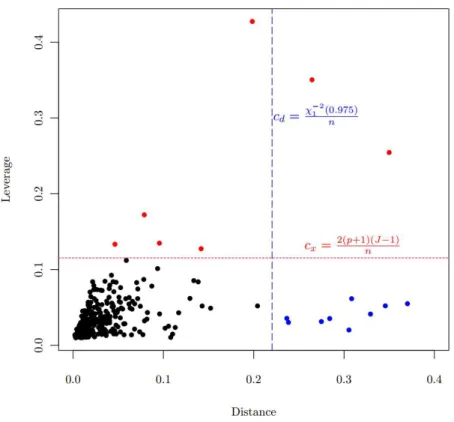
Figure 1 Scatter plot of distance vs. leverage, which are based on MLE.Criteriacdfor the distance and

cxfor the leverage are demonstrated.

Table 1 Summary statistics for surveyed subjects.

Covariate Hypertension categories

Normal Pre-hypertension Stage 1 Stage 2

Gender Male 138 104 29 8

Female 87 114 31 9

Age Mean 43.2 48.8 54.3 60.3

Std. Dev. 13.7 13.8 12.2 13.4

BMI Mean 43.2 48.8 54.3 60.3

Std. Dev. 13.7 13.8 12.2 13.4

Sodium intake Mean 3.7 3.7 4.6 2.7

Std. Dev. 3.0 2.4 5.0 2.1

for the odds between the Pre-hypertension and the Normal categories. The scatter plot (Fig. 1) between distances and leverages suggests some observations are possible outliers: Observations 21, 33, 85, 92, 194, 274, 336, 414, 459, 483, and 489 have large distances, which are blue-colored, and Observations 37, 83, 263, 459, 483, 485, and 490 have large leverages, which are red-colored.

Figure 2 Compare odds plots of sodium intakes between MLE estimates and GMWM estimates on the population of female, age=40, and BMI=23.

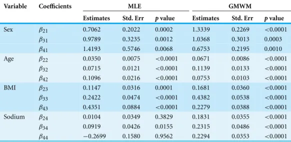
Table 2 Polytomous logistic regression of a hypertension data: coefficient estimates and standard errors from GMWM and MLE.

Variable Coefficients MLE GMWM

Estimates Std. Err pvalue Estimates Std. Err pvalue

Sex β₂₁ 0.7062 0.2022 0.0002 1.3339 0.2269 <0.0001

β31 0.9789 0.3235 0.0012 1.0368 0.3013 0.0003

β₄₁ 1.4193 0.5746 0.0068 0.6753 0.2195 0.0010

Age β22 0.0350 0.0075 <0.0001 0.0671 0.0086 <0.0001

β32 0.0715 0.0121 <0.0001 0.1139 0.0133 <0.0001

β42 0.1096 0.0216 <0.0001 0.0753 0.0103 <0.0001

BMI β23 0.1147 0.0316 0.0001 0.1681 0.0360 <0.0001

β₃₃ 0.2422 0.0474 <0.0001 0.4382 0.0538 <0.0001

β43 0.4351 0.0884 <0.0001 0.2279 0.0388 <0.0001 Sodium β₂₄ 0.0104 0.0349 0.3829 0.1831 0.0355 <0.0001

β34 0.0919 0.0426 0.0155 0.2315 0.0486 <0.0001

β44 −0.2699 0.1580 0.9562 0.2294 0.0353 <0.0001

Notes.

Std. Err, standard error.

MATERIALS AND METHODS

The baseline-category logit model

Assume a random sample of sizenfrom a large population. Each element in the population may be classified into one ofJcategories, denoted byyi=(yi1,yi2,...,yiJ)the multinomial trial for subjecti, whereyij=1 when the response is in categoryjandyij=0 otherwise, i₌1,...,n,j₌1,...,J. Thus,

jyij =1. Supposepexplanatory covariates, with at least one of them being continuous, are observed. Definexi =(1,xi1,...,xip), and

x=(x1,...,xn). We assume that(yi,xi)are independently and identically distributed (i.i.d.). Letπij =πj(xi)=P(Yi =j|xi), denote the probability that the observation of Y belongs to categoryj, given covariatesxi, we assume the relationship between the probabilityπjandxcan be modeled as:

log _π

j(xi)

πJ(xi) 

=xT_i βj, j=2,...,J (1)

whereβ_jT ₌(βj0,βj1,...,βjp). Here we set the first category as reference class. This model is called a baseline-category logit model (Agresti, 2012) or generalized logit model (Stokes, Davis & Koch, 2009). MLE is usually used for obtaining parameter estimation of this model. Here we present an alternative estimation method formed with the GMM.

Estimation using GMM

The baseline-category logit model can be viewed as a multivariate model. Definey∗_iT₌

(yi2,...,yiJ), sinceyi1is redundant. LetXT=(X1T,...,XnT)is an(J−1)×(p+1)(J−1) matrix, withX_iT, a(J₋1)_×(p₊1)(J₋1)matrix, defined as:

XT_{i =} 

   

xT_i xT_i

···

xT_i 

   

. (2)

In the GMM framework, we define

u(β)₌Xi(yi∗−πi), i=1,...,n (3)

whereπT_{i =}(πi2,πi3,...,πiJ). AndβT=(β2T,β3T,...,βJT)is the(p+1)(J−1)vector of unknown parameters. The population moment condition is

E_{u(β)_{} =}0,

with the corresponding sample moment condition

Un(β)= n 

i=1

The GMM estimation ofβˆM can be obtained by minimizing the following quadratic objective function

Qn(β)=UnT(β)Σn−1(β)Un(β),

whereΣn(β)can be the empirical variance–covariance matrix given by

Σn(β)= 1 n2

n 

i=1

uT(β)u(β)₋1

nUn(β)U T n(β).

Or, for the best efficiency of the GMM estimation, we can take the information matrix of the polytomous logit model (PLRM), that is,

Σn(β)= n 

i=1

Xi(Di−πiπTi )XiT (5)

whereDi=diagonal(πi).

In general,βˆMcan be computed via an iterative procedure (Hansen, Heaton & Yaron, 1996). Under standard regularity conditions, the GMM estimatorβMˆ exists and converges in probability to the true parameterβ0(Hansen, 1982). A proof of asymptotic normality of GMM can be found on p. 2148 ofNewey & McFadden (1994).

A robust GMM

In this section we introduce the outlier robust GMM estimator. In the following subsection, we specify moment conditions used for robust estimation. And the details on the implementation of the estimator follows.

The generalized method of weighted moments

The main principle used in the robust GMM estimator is that we replace moment conditions by a set of observation weighted moment conditions. Instead ofEq. (3), we define

uw(β)₌wiXi(yi∗−πi)−ci, i=1,...,n (6)

whereci=E{wiXi(y∗_i −πi)}. Then the estimation can be based on the moment conditions

E{uw(β)_{} =}0.

Consequently, the generalized method of weighted moments (GMWM) estimates can be defined by

ˆ

βw₌argmin

β∈BQ w

n(β) (7)

where

with

U_nw(β)₌

n 

i=1

uw(β). (9)

Here we take the summation as the sample moment condition. The advantage of using the summation is that it can lead us to a direct estimation of covariance matrix.

It is clear to see that this definition is analogous to the standard GMM. If we choose wi =1 andci =0 for all observations, the moment conditions in(6)are reduced to the standard moment conditions. Therefore, the standard GMM is a special case of the GMWM.

In order to specify the weights for the robust GMM estimator, we need the following definition of a distance, which is based on individual moment conditions:

di(β)= [uwi (β)]T{Σwn(β)}−1uwi (β), i=1,...,n. (10)

The weight is assigned based ondi(β), that is,wd=w 

di(β). There are several alternative specifications of weight functions available in the literature (Huber, 1981;Hampel et al., 2005). In this study, the Huber’s weights are applied:

w

di(β)=min 

1, cd

di(β) 

. (11)

The above specification of weight function requires a value of the tuning constantcd. Both the outlier sensitivity and the efficiency of the estimator are determined by the constant. On the one hand, the estimator should be reasonably efficient if the sample contains no outlier. On the other hand, the estimator should be insensitive to outliers. To determine cd, understanding the distribution ofdi(β)is critical. Clearly,uw_i (β)is a column vector, anddi(β)is a scalar quadratic distance, so we setcd=χ1−2(0.975)/n, whereχp−2(·)is the quantile of theχ2distribution withpdegrees of freedom.

If we take the information matrix(5)of the PLRM asΣ_nw(β), we can compute leverage for each observation:

Hi=Xi{Σnw(β)}−1XiTσiw, i=1,...,n (12)

whereσ_iwis theith component ofΣw_n(β). Then, a Mallows-type weight can be defined based ontrace(Hi); that is,wx=w(trace(Hi)), to downplay the observations with high leverages.Lesaffre & Albert (1989)suggest that the practical rule for isolating leverage points might setcx=2(p+1)(J−1)/n. In this study, we give observations with large leverages 0 weights,

wx=w(trace(Hi))=  



1 iftrace(Hi)≤

2(p₊1)(J₋1)

n 0 otherwise.

(13)

The consistency correction vectorciis defined as

ci= 

wd_i(1)(β)



−wd_i(0)(β)



/diag

Σ_nw(β), i₌1,...,n

wherewd_i(h)(β)



=wXi{h−πi(β)}/diagΣnw(β) −1

withh_{= {}0,1_}, is the weight for y_i∗.

Implementation of the estimator

The continuous updating estimation method is applied in this study for estimating the regression coefficients and corresponding variance. The procedure is detailed as follows:

1. Apply an initial valueβ(0)for computingΣn 

β .

2. Computedi(β)usingEq. (10)andHiusingEq. (12); assign weights correspondingly based on(11)and(13).

3. With the combined weights, calculateΣ_nw(β)andU_nw(β)inEq. (9). 4. Obtain the estimatorβˆ(w1)by minimizingQwnofEq. (8).

5. Go back to Step 1, replaceβ(0)with the estimatorβˆ(w1)in computingΣnw 

ˆ

β(w1) 

, and move to the next iteration.

6. Continue this procedure until convergence criteria are met.

For the starting valueβ(0), a reasonable choice is the MLE estimation based on the original data.

In the appendix, we proved that, under some regularity assumptions, we can have that

ˆ

βwis consistent forβ0. And by studying the behavior of the weighted moment equations in a neighborhood ofβ0, we showed that the asymptotic linearity ensures the applicability of the central limit theorem for the asymptotic normality of GMWM.

RESULTS

Monte Carlo simulations

In this section we investigate the properties of the GMWM estimator using a Monte-Carlo study. We generate data with three response categories and two covariates which are from multivariate normal distribution with 0 mean and identity covariance. The true coefficient matrixβ0is

β0= 

 

β10 β20 β30

β11 β21 β31

β12 β22 β32 

 =



 

0 1.0 ₋0.3 0 −0.8 0.7 0 ₋1.0 ₋0.5



 .

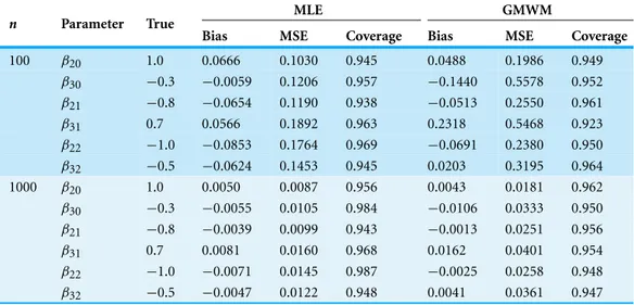
Table 3 Bias of parameter estimates and MSE from randomly generated data without outliers.

MLE GMWM

n Parameter True

Bias MSE Coverage Bias MSE Coverage

100 β20 1.0 0.0666 0.1030 0.945 0.0488 0.1986 0.949

β30 −0.3 −0.0059 0.1206 0.957 −0.1440 0.5578 0.952

β21 −0.8 −0.0654 0.1190 0.938 −0.0513 0.2550 0.961

β31 0.7 0.0566 0.1892 0.963 0.2318 0.5468 0.923

β_{22 −}1.0 −0.0853 0.1764 0.969 −0.0691 0.2380 0.950

β32 −0.5 −0.0624 0.1453 0.945 0.0203 0.3195 0.964

1000 β₂₀ 1.0 0.0050 0.0087 0.956 0.0043 0.0181 0.962

β30 −0.3 −0.0055 0.0105 0.984 −0.0106 0.0333 0.950

β21 −0.8 −0.0039 0.0099 0.943 −0.0013 0.0251 0.956

β31 0.7 0.0081 0.0160 0.968 0.0162 0.0401 0.954

β22 −1.0 −0.0071 0.0145 0.987 −0.0025 0.0258 0.948

β_{32 −}0.5 −0.0047 0.0122 0.948 0.0041 0.0361 0.947

are generated usingrmultinorm(ni,Ni,π(xi))function, whereπ(xi)=(π1(xi),...,πJ(xi)) is the probability vector,niis the number of random vectors to draw, andNiis the total number of objects that are put intoJ-categories. In our case,ni=Ni=1 for all subjects andJ=3.

Two sample sizes, 100 and 1000, are examined. For each sample size, we run the simulation 1000 times. Average biases and MSEs are calculated and tabulated.Table 3

shows the results from randomly generated data with no outliers added. When the sample size is small, GMWM will give greater biases onβ30andβ31compared to the MLE method. For the sample size 1000, biases on these two parameters increase too, but not so obviously. Variances will also be inflated due to the weights we applied.

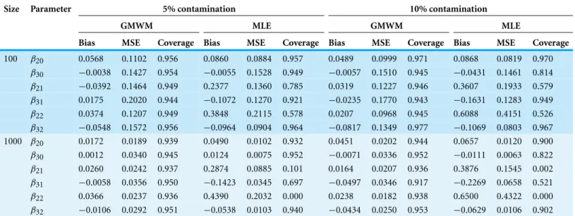
Outliers are generated from a multivariate normal distribution with the mean vector

=(2,3)and identity covarianceI2. For these outliers, their responses are intentionally misclassified, that is, they are placed within a different category from those predicted categories based on the true parameters.

Table 4lists simulation results with outliers added. For estimations from datasets with 5% outliers, bias correction from the GMWM is excellent. However, when the datasets have 10% outliers, biases on estimations of some parameters (β21andβ22in this simulation) are decreased, but not completely corrected.

Application

Table 4 Comparison between GMWM and MLE estimation from randomly generated data with outliers added.

Size Parameter 5% contamination 10% contamination

GMWM MLE GMWM MLE

Bias MSE Coverage Bias MSE Coverage Bias MSE Coverage Bias MSE Coverage

100 β20 0.0568 0.1102 0.956 0.0860 0.0884 0.957 0.0489 0.0999 0.971 0.0868 0.0819 0.970

β30 −0.0038 0.1427 0.954 −0.0055 0.1528 0.949 −0.0057 0.1510 0.945 −0.0431 0.1461 0.814

β21 −0.0392 0.1464 0.949 0.2377 0.1360 0.785 0.0319 0.1227 0.946 0.3607 0.1933 0.579

β31 0.0175 0.2020 0.944 −0.1072 0.1270 0.921 −0.0235 0.1770 0.943 −0.1631 0.1283 0.949

β₂₂ 0.0374 0.1207 0.949 0.3848 0.2115 0.578 0.0207 0.0968 0.945 0.6088 0.4151 0.526

β32 −0.0548 0.1572 0.956 −0.0964 0.0904 0.964 −0.0817 0.1349 0.977 −0.1069 0.0803 0.967 1000 β₂₀ 0.0172 0.0189 0.939 0.0490 0.0102 0.932 0.0451 0.0202 0.944 0.0657 0.0120 0.900

β30 0.0012 0.0340 0.945 0.0124 0.0075 0.952 −0.0071 0.0336 0.952 −0.0111 0.0063 0.822

β21 0.0260 0.0242 0.937 0.2874 0.0885 0.101 0.0164 0.0207 0.936 0.3876 0.1545 0.002

β31 −0.0058 0.0356 0.950 −0.1423 0.0345 0.697 −0.0497 0.0346 0.917 −0.2269 0.0658 0.521

β22 0.0366 0.0237 0.936 0.4390 0.2032 0.000 0.0238 0.0182 0.938 0.6500 0.4322 0.000

β_{32 −}0.0106 0.0292 0.951 −0.0538 0.0103 0.940 −0.0434 0.0250 0.953 −0.0629 0.0106 0.902

inconsistencies: the coefficient of sodium intake for the odds model between the Stage 2 hypertension and the Normal categories is no longer negative, see the right side ofTable 2.

As the results indicate, age, gender, and BMI all had significant impact on hypertension status. For example, one unit increase in BMI resulted in an increase of 1.26 (95% confidence interval [1.16–1.35]) times in likelihood to have Stage 2 hypertension when compared with the normal status. And with one year age increase, a subject was 1.07 (95% CI [1.06–1.10]) times more likely to have Stage 2 hypertension than to stay at the normal healthy status. Contrary to the MLE results for sodium intakes, which were difficult to make a conclusion due to inconsistent estimate, we now find that sodium intakes were statistically significant. When a daily intake of sodium increased one gram, a subject were 1.26 (95% CI [1.15–1.37]) times more likely to have Stage 1 hypertension, and 1.25 (95% CI [1.17–1.35]) times more likely to have Stage 2 hypertension. These results are consistent with the findings from previous studies (National Research Council, 2005;He & MacGregor, 2004).

DISCUSSION

A reasonable choice to fit ordinal response data is the proportional odds model if the proportional odds assumption is not violated. Proportional odds models can take the ordinal information into modeling. And it reduces the number of parameters which is needed by the generalized logit model. Unfortunately, our data does not met the fundamental assumption of proportional odds models, which makes us choose to treat the outcome as a nominal response.

conditions with weighted moment conditions, so that aberrant observations automatically receive less weight. We proved that the proposed method has good asymptotic behavior. When outliers are present, the GMWM estimator give much smaller biases than the estimations derived from the traditional MLE method. This method can be adapted to check whether results obtained with the traditional MLE approach are driven only by a few outlying observations. The weights produced from the robust procedure can be used to diagnose the cause of the differences and to indicate routes for model re-specification.

APPENDIX: CONSISTENCY AND ASYMPTOTIC

NORMALITY

In this appendix, we introduce the assumptions for the asymptotic analysis of GMWM, and outline the derivations on the main asymptotic properties of GMWM.

We make the following sets of regularity assumptions regarding properties of the moment functions and identification assumptions.

Assumption I

I1. B_{is a compact parametric space.} I2. Σis a positive definite matrix.

I3. It holds thatE_[uw(β)_{] =}0 if and only ifβ₌β0, and for anyϵ >0, that

inf

β∈B\N(β0,ϵ) 

E[uw(β)]  >0

whereN_{(β0,ϵ)= {β∈R}l

∥β−β₀∥< ϵ}is an openϵ-neighborhood of a pointβ₀.

Assumption F

F1. Letuw(β)be continuous inβ∈B_{, and be twice differentiable inβon}N(β0,ϵ)almost surely.

F2. Expectation Esup_β∈B  uw(β)



, Esup_β∈N(β 0,ϵ)



∂uw(β)/∂β_k  , and

Esup_β∈N(β0,ϵ) 

∂2uw(β)/∂β_k∂β_l 

exists and are finite fork,l=1,...,p.

Assumption W

W1. limϵ_→0sup_∥Δ∥≤ϵ|w(β+Δ)−w(β)| =0.

W2. limϵ_→0sup_∥Δ_∥≤ϵ|∂w(β+Δ)/∂β−∂w(β)/∂β| =0.

When the above assumptions are met, we can prove thatβwˆ is consistent forβ0. We begin with studying the behavior of the weighted moment equations in a neighborhood ofβ0. And proving their asymptotic linearity is followed. The linearity ensures the applicability of the central limit theorem for the asymptotic normality of GMWM.

Theorem 1.Let the assumptionsFandIhold, then the GMWM estimatorβˆwis asymptoti-cally normal, that is,√nβwˆ ₋β0

 _F

−→N(0,MTSwM)as n_{→ ∞}, where

Sw=E  1 n n 

i=1

uw(βˆ)uw(βˆ)T



with Vw=E 

∂Uw_(β)ˆ

∂βT 

.

We start with proving two lemmas before we present the proof ofTheorem 1. Lemma 1.Let the assumptionsF,IandWhold, and let U_rw(β)be the rthelement of the vector Uw(β), r₌1,...,p. Then, for0<s<1,

sup

∥t∥≤C      1 n  i p 

l=1 tl



(∂/∂βl)Uiw,r 

β_+√st n



−(∂/∂βl)Uiw,r(β) _

  

=op(1). (14)

Proof.Forl,r₌1,...,p, by differentiating theith component ofU_rw(β), we get

∂U_iw_,r(β)

∂βl = − w(β)Xi

∂πi(β)

∂βl +

∂wi(β)

∂βl

Xi(yi−πi(β)).

Then,

sup

∥t∥≤C      1 n n 

i=1

p 

l=1 tl



(∂/∂βl)Uiw,r 

β_+√st n



−(∂/∂βl)Uiw,r(β) _    ≤ C n n 

i=1

p 

l=1 tl sup

∥t∥≤C    

(∂/∂βl)U_iw,r 

β_+√st n



−(∂/∂βl)U_iw,r(β)     and sup

∥t∥≤C    

(∂/∂βl)Uiw,r 

β_+√st n



−(∂/∂βl)Uiw,r(β)    

≤ sup

∥t∥≤C 

  wi

 β_+√st

n 

−wi  β     

∂/∂βl)πi 

β_+√st n      + sup

∥t∥≤C 

  

(∂/∂βl)πi 

β_+√st n



−(∂/∂βl)πi 

β    |Xiwi

 β

|



+ sup

∥t∥≤C 

  

(∂/∂βl)wi 

β_+√st n



−(∂/∂βl)wi  β        Xi

 yi−πi

 β_+√st

n      + sup

∥t∥≤C 

   

yi−πi 

β_+√st n



− yi−πi

 β     

∂/∂βl)wi 

β  

.

Then, by taking expectation at both sides,

E 

sup

∥t∥≤C    

(∂/∂βl)Uiw,r 

β_+√st n



−(∂/∂βl)Uiw,r(β)      ≤ sup

∥t∥≤C    wi

 β_+√st

n 

−wi  β     sup

∥t∥≤C 

∂/∂βl)πi 

β_+√st n

+ sup

∥t∥≤C    

(∂/∂βl)πi 

β_+√st n



−(∂/∂βl)πi  β     sup

∥t∥≤C| Xiwi

 β

|

+ sup

∥t∥≤C    

(∂/∂βl)wi 

β_+√st n



−(∂/∂βl)wi  β    E  sup

∥t∥≤C    Xi

 yi−πi

 β_+√st

n      + sup

∥t∥≤C     

yi−πi 

β_+√st n



−

yi−πiβ    

sup

∥t∥≤C 

∂/∂βl)wiβ.

Thus, by conditionsFandW, we have

E 

sup

∥t∥≤C    

(∂/∂βl)Uiw,r 

β_+√st n



−(∂/∂βl)Uiw,r(β)     

−→0, _∀i

and

E 

sup

∥t∥≤C      1 n n 

i=1

p 

l=1 tl



(∂/∂βl)Uiw,r 

β_+√st n



−(∂/∂βl)Uiw,r(β) _

   

−→0, _∀i.

Therefore, we have the results in(14).

Lemma 2.Let the assumptionsF,IandWhold, it holds that

1

√

n_∥supt∥≤C   U

w

n(β0+n−

1

2_t)−_Uw

n(β0)+Vwn−

1 2_t

 

=op(1), (15)

as n_{→ ∞}, where Vw₌E∂U_∂βwT(β) 

. Proof.Write

U_nw(β0+n−

1

2_t)−_Uw n(β0)=

n 

i=1

wi(β0+n−

1

2_t)ui(β₀+_n− 1 2_t)−

n 

i=1

wi(β0)ui(β0).

By the Taylor expansion,ui(β0+n−

1

2_t)=_ui(β₀₎+_n−12_t 

∂

∂βui(β0+√tn) 

, where 0<s<1. Then, we can write

U_nw(β0+n−

1

2t₎−Uw n(β0)

=

n 

i=1 ui(β0)



wi(β0+n−

1

2t₎−w_i(β₀₎ 

(16)

+√1

n n 

i=1

wi(β0)t

∂

∂βui(β0) (17)

+√1

n n 

i=1 

wi(β0+n−

1

2_t)−_wi(β₀₎ 

t ∂

∂βui(β0) (18)

+√1

n n 

i=1 wi

 β0+

t √ n  t   

∂ui 

β0+√t_n 

∂β −

∂ui(β0)

∂β  



We will now show that terms(16),(18)and(19)are asymptotically negligible. As to the term(16), By assumptionW1,_{wi(β0+n−

1

2t₎−w_i(β₀₎} →0, andu_i(β₀₎is independent ofβ. So we have the term(16)tends to zero. Similarly,∂/∂βui(β0)is independent ofβandt

is bounded. Hence, the term(18)tends to zero.Lemma 1implies∂ui 

β0+√t_n 

∂β − ∂ui(β0)

∂β →0,

asn→ ∞. So the term(19)can be neglect too.

Now, let us analyze the term(17). Letw∗_i(β0)be the limit ofwi(β0). Rewrite(17)as

1

√

n n 

i=1

wi(β0)t

∂

∂βui(β0)= 1

√

n n 

i=1 

wi(β0)−wi∗(β0) 

t ∂

∂βui(β0) (20)

+√1

n n 

i=1 

w∗_i(β0)t

∂

∂βui(β0)−E 

w_i∗(β0)t

∂ ∂βui(β0)

 (21)

+√1

nE 

w_i∗(β0)t

∂ ∂βui(β0)



. (22)

The first term(20)is negligible because∂/∂βui(β0)is independent ofβ,tis bounded, and

wi(β0)−w_i∗(β0)→0. By the central limit theorem, each element of vector(21) converges in distribution to a normally distribution random variable with zero mean and a finite variance which is uniformly bounded byt. Hence,(21)is bounded in probability. The last term(20)is

1

√

nE 

w∗_i(β0)t

∂ ∂βui(β0)



= √t

nV w_.

This proves the lemma.

Proof of Theorem 1.Sincetn=√n=Op(1)asn→ ∞byLemma 2, we can write(15)as

U_nw(β0+n−

1

2_tn)−Uw

n(β0)+Vwn−

1

2_tn=op(n−12_{) (23)}

with a probability arbitrarily close to one uniformly intn∈ {t: ∥t∥ ≤C}. Moreover, with n−12_tn=_op(1),∂Uw

n(β0+n−

1

2_tn)/∂β→_Vw_{in probability asn}→ ∞_. Note that the first order conditions of GMWM equal to 0, that is,

∂Qw_n(βw)

∂β = 

∂U_nw(βw)

∂β T

Σ(βw)U_nw(βw)₌0.

ReplaceU_nw(βw)withU_nw(β0+n−

1

2t_n)fromEq. (23),



∂U_nw(β0+n−

1 2_tn)

∂β

T

Σ(βw)U_nw(β0+n−

1 2_tn)

=

Vw+op(1) T

Σ(βw) 

U_nw(β0)−Vwn−

1 2_tn



=0.

Then we have

tn=√n(βw−β0)=√n 

Next we examine the behavior of√nU_nw(β0), which can be written as

√

nU_nw(β0)=n−

1 2

n 

i=1

ui(β0)wi(β0)

=n−12 n 

i=1

ui(β0)wi(β0)−w_i∗(β0) (25)

+n−12 n 

i=1

ui(β0)w∗_i(β0). (26)

Note that the term(25)is asymptotically negligible in probability due to the triangle in-equality and assumptionW1. The term(26)is a stationary sequence of absolutely random variables. By assumptionI3andF2,(26)have zero mean and finite second moments. So the central limit theorem can be applied on(26), giving√nU_nw(β0)∼N(0,Sw)(Davidson,

1994, Section 25.3)

WithEq. (24), we have asymptotic normality ofβw, and its asymptotic variance is given

byMTSwM(Davidson, 1994).

ADDITIONAL INFORMATION AND DECLARATIONS

Funding

No funding was provided for this work.

Competing Interests

Xiaoshan Wang is an employee of the Center For Clinical And Translational Research, Forsyth Institute.

Author Contributions

• Xiaoshan Wang conceived and designed the experiments, performed the experiments, analyzed the data, contributed reagents/materials/analysis tools, wrote the paper, prepared figures and/or tables, reviewed drafts of the paper.

REFERENCES

Agresti A. 2012.Categorical data analysis. New Jersey: Wiley.

Baum CF, Schaffer ME, Stillman S. 2002.Instrumental variables and gmm: estimation and testing. Boston College Working Papers in Economics 545, Boston College Department of Economics.

Copas JB. 1988.Binary regression models for contaminated data.Journal of the Royal Statistical Society Series B (Methodological)50:225–265.

Davidson J. 1994.Stochastic limit theory: an introduction for econometricicans,Advanced texts in econometrics.New York: Oxford University Press.

Gupta A, Kasturiratna D, Nguyen T, Pardo L. 2006.A new family of ban estimators for polytomous logistic regression models based onφ-divergence measures.Statistical Methods & Applications15:159–176DOI 10.1007/s10260-006-0008-6.

Hampel FR, Ronchetti EM, Rousseeuw PJ, Stahel WA. 2005.Robust statistics: the approach based on influence functions. New York: Wiley-Interscience.

Hansen LP. 1982.Large sample properties of generalized method of moments estimators.

Econometrica50:1029–1054DOI 10.2307/1912775.

Hansen LP, Heaton J, Yaron A. 1996.Finite-sample properties of some alternative gmm estimators.Journal of Business & Economic Statistics14:262–280.

Hayashi F. 2000.Econometrics. New Jersey: Princeton University Press.

He FJ, MacGregor GA. 2004.Effect of longer-term modest salt reduction on blood pressure.

Cochrane Database of Systematic Reviews(3): CD004937.

Heritier S, Cantoni E, Copt S, Victoria-Feser MP. 2009.Robust methods in biostatistics. New Jersey: Wiley.

Huber PJ. 1981. Robust statistics, Wiley series in probability & statistics.New York: Wiley-Interscience.

Kuersteiner GM. 2012.Kernel-weighted GMM estimators for linear time series models.Journal of Econometrics170:399–421DOI 10.1016/j.jeconom.2012.05.013.

Lesaffre E, Albert A. 1989.Multiple-group logistic regression diagnostics.Journal of the Royal Statistical Society Series C (Applied Statistics)38:425–440.

Liu I, Agresti A. 2005.The analysis of ordered categorical data: an overview and a survey of recent developments.TEST14:1–73DOI 10.1007/BF02595397.

McCullagh P, Nelder JA. 1989.Generalized linear models,Chapman & Hall/CRC monographs on statistics & applied probability,second edition. London: Chapman and Hall/CRC.

Mebane JWR, Sekhon JS. 2004.Robust estimation and outlier detection for overdispersed multinomial models of count data. American Journal of Political Science48:392–411 DOI 10.1111/j.0092-5853.2004.00077.x.

National Research Council. 2005.Dietary reference intakes for water, potassium, sodium, chloride, and sulfate. Washington, DC: The National Academies Press.

Newey WK, McFadden D. 1994.Large sample estimation and hypothesis testing. In: Engle R, McFadden Dan, eds.Handbook of econometrics, Vol. 4. Amsterdam: North Holland.

Newey WK, West KD. 1987.Hypothesis testing with efficient method of moments estimation.

International Economic Review28:777–787DOI 10.2307/2526578.

Pakes A, Pollard D. 1989. Simulation and the asymptotics of optimization estimators.

Econometrica57:1027–1057DOI 10.2307/1913622.

Pregibon D. 1982.Resistant fits for some commonly used logistic models with medical applications.Biometrics38:485–498DOI 10.2307/2530463.

Ronchetti E, Trojani F. 2001.Robust inference with gmm estimators.Journal of Econometrics 101:37–69DOI 10.1016/S0304-4076(00)00073-7.

Rousseeuw PJ, Leroy AM. 2003. Robust regression and outlier detection. New York: Wiley-Interscience.

Stokes ME, Davis CS, Koch GG. 2009.Categorical data analysis using the SAS system. North Carolina: SAS Institute.