Axial-Flow Compressor Performance Prediction in Design and Off-Design Conditions through 1-D and 3-D Modeling and Experimental Study

J_{ournal of} A_pplied F_luid M_{echanics, Vol. 9, No. 5, pp. 2149-2160, 2016.} Available online at www.jafmonline.net, ISSN 1735-3572, EISSN 1735-3645.

Axial-Flow Compressor Performance Prediction in

Design and Off-Design Conditions through 1-D

and 3-D Modeling and Experimental Study

A. Peyvan and A. H. Benisi

†

School of Mechanical Engineering, Sharif University of Technology, Tehran, Iran

†Corresponding Author Email: Hajilouy@ sharif.edu

(Received June 28, 2015; accepted December 11, 2015)

A

BSTRACT

In this study, the main objective is to develop a one dimensional model to predict design and off design performance of an operational axial flow compressor by considering the whole gas turbine assembly. The design and off-design performance of a single stage axial compressor are predicted through 1D and 3D modeling. In one dimensional model the mass, momentum and energy conservation equations and ideal gas equation of state are solved in mean line at three axial stations including rotor inlet, rotor outlet and stator outlet. The total to total efficiency and pressure ratio are forecasted using the compressor geometry, inlet stagnation temperature and stagnation pressure, the mass flow rate and the rotational speed of the rotor, and the available empirical correlation predicting the losses. By changing the mass flow rate while the rotational speed is fixed, characteristic curves of the compressor are obtained. The 3D modeling is accomplished with CFD method to verify one dimensional code at non-running line conditions. By defining the three-dimensional geometry of the compressor and the boundary conditions coinciding with one three-dimensional model for the numerical solver, axial compressor behavior is predicted for various mass flow rates in different rotational speeds. Experimental data are obtained from tests of the axial compressor of a gas turbine engine in Sharif University gas turbine laboratory and consequently the running line is attained. As a result, the two important extremities of compressor performance including surge and choking conditions are obtained through 1D and 3D modeling. Moreover, by comparing the results of one-dimensional and three-dimensional models with experimental results, good agreement is observed. The maximum differences of pressure ratio and isentropic efficiency of one dimensional modeling with experimental results are 2.1 and 3.4 percent, respectively.

Keywords: Axial compressor; One dimensional modeling; Three dimensional modeling; Characteristic curve.

N

OMENCLATURE

A

cross section area

C

absolute velocity

Ca

axial velocity

p

C

constant pressure specific heat capacity

c

profile chord

D

diffusion factor

i

incidence angle(degree)

sh

K

blade shape parameter

, t i

K

design incidence angle thickness

correction factor

, t

K

design deviation angle thickness

correction factor

L

stagnation temperature to static

temperature ratio

M

Mach number



density



cp/cv



absolute angle(degree)



relative angle(degree)



loss coefficient



quantity difference



work done factor



deviation angle(degree)



camber angle(degree)



solidity



dimensionless incidence angle

Super script

*

design condition

Sub script

Mp

mass parameter

m

slop parameter

m

mass flow rate

N rotational speed of rotor

P

pressure

R

gas constant

r

radius

res

residual

s

entropy

T temperature

t

airfoil thickness

j

u

rotor linear velocity

W

relative velocity

rotor outlet station

stator outlet station

pro

profile

end

end-wall

clear

clearance

shock

shock

ps

positive stall

ns

negative stall

max

maximum

eq

equivalent

rel

relative

1.

I

NTRODUCTION

Axial flow compressor performance prediction is associated with the complexities and difficulties. Many studies have been conducted on the various components of the axial compressor but a general model that can predict the performance specifications of various types of axial flow compressors with good accuracy is needed (Howell and Calvert 1978; Wennerstrom 1990). Although, many theoretical and experimental models have been developed to predict different losses of axial compressor, including incidence and deviation angles for design and off design conditions, incidence angles for negative and positive stall conditions, and stall onset, common existing experimental models have been obtained from experiments on a specific compressor and since the flow field dramatically changes due to a slight change in geometry, or in component connected to the compressor or in gas turbine configuration, a presented experimental correlation may not provide good results for other cases. Furthermore, in the most performance prediction studies, axial compressor has been treated as an isolated component. However, this study focuses on an operating axial compressor of a gas turbine engine. In fact, a one-dimensional model, which predicts the performance of an operational compressor and its results are verified with experimental results,can be used to redesign or improve the performance of the compressor of the gas turbine system. Also, it is plausible to use 1D modeling for parameter study because it is so fast.

Lieblein (1965) tested two-dimensional cascade in order to calculate blade profile loss using the definition of equivalent diffusion coefficient. He could also obtain correlation to predict incidence and deviation angles for the design point. Bullock and Johnsen (1965) studied design incidence and deviation angles and they offered a model for calculating these angles at design point. Herrig et al. provided an approximate equation to calculate the positive and negative stall angles for NACA 65 series blades. The equation was obtained from a series of two-dimensional cascade test results with low Mach number Aungier (2003). Koch and Smith (1976) conducted extensive studies on various

compressors and succeeded to develop Lieblein’s model and provided more accurate model to estimate the blade profile loss. Another important source of energy loss in axial compressor is wall boundary layer on which Koch and Smith (1976) conducted extensive studies and proposed accurate model to predict the pressure loss. By modifying the correlation which predicts the pressure loss related to tip clearance of centrifugal compressor, Aungier (2003) was able to predict tip clearance loss of rotor of axial flow compressor.

According to distortion of flow during the off-design performance of the compressor, it is difficult to develop a model to predict the performance. In this context, Bullock and Johnson (1965) proposed an empirical relationship to calculate the deviation angle of off-design condition. Aungier (2003) introduced the normalized incidence angle to calculate the overall loss coefficient in off-design condition.

All the aforementioned models as well as the secondary flow loss of Howell (1958) are used for 1D modeling in this research.

Madadi and Hajilouy (2008) developed one-dimensional model to predict design and off-design performance of two stage axial compressor. However the case study, NASA compressor, was an isolated compressor without considering the whole assembly of gas turbine system.

Song et al. (2001) provided a performance predicting method which differs from the conventional sequential stage-stacking method in which it employs simultaneous calculation of all interstage variables like temperature, pressure and flow velocity. The effect of interstage air bleeding on compressor performance is also demonstrated on their work.

Garzon and Darmofal (2003) used a probabilistic methodology to investigate the impact of geometry on compressor performance. They applied a mean-line multistage compressor modelwith probabilistic loss and turning models from the blade-passage analysis to quantify the blade geometry effects on pressure ratio and efficiency.

gas turbine performance which uses compressor and turbine performance maps obtained by using generalized stage performance curves matched by means of the “stage–stacking” procedure. The overall multistage compressor performance is predicted using generalized relationships between stage efficiency, pressure coefficient and flow coefficient.

Here, because the tests are performed on an axial compressor within a gas turbine engine, only the running line could be obtained because it is impossible to change the mass flow rate while the rotational speed of the engine is fixed. Therefore, for each rotational speed there is only a single point to compare and validate the one-dimensional modeling results. To compare and verify the modeling results for non-running line conditions, a CFD modeling is applied using a verified commercial code.

Three-dimensional modeling is performed using computational fluid dynamics. Having three-dimensional geometry of the compressor, it is meshed. Overall number of grid for rotor and stator domain is about 500,000. Then the boundary conditions are defined. In this process, turbulence model and flow are considered to be k-epsilon and compressible, respectively. Total pressure and total temperature are specified as rotor inlet boundary conditions and mass flow rate is specified for stator outlet. In each rotational speeds, by solving the flow field with different mass flow rates, the characteristic curves of the compressor are obtained.

The experiments have been done for an axial compressor embedded in a gas turbine in Gas Turbine laboratory of Sharif University. There are several measuring stations on gas turbine engine and only the first four of them are used for this study including bell mouth throat, axial compressor rotor inlet and outlet and finally axial compressor stator outlet. At these stations, the stagnation and static pressures and temperatures as well as the engine speed and mass flow rate are measured. All measuring devices are calibrated prior to tests and actual values are calculated using calibration curves.

2.

O

NE

-D

IMENSIONAL

M

ODELING

One dimensional modeling is performed to predict design and off-design performance of the axial compressor.

For one dimensional modeling, equations of conservation of mass, momentum, and energy, as well as equations of ideal gas, second law of thermodynamics, the energy losses and predicted deviation angles in design and off-design conditions are solved together on mean radius of compressor blades in order to determine the air flow unknowns.

2.1

Assumptions

Main assumptions of 1D modeling are as below:

1. Air flow properties changes are ignored in

radial and circumferential directions.

2. Constant pressure specific heat coefficient change is neglected.

3. In design condition, inlet flow collides the blade at design incidence angle.

4. Flow viscosity doesn’t change due to small variations of temperature.

2.2

Inputs

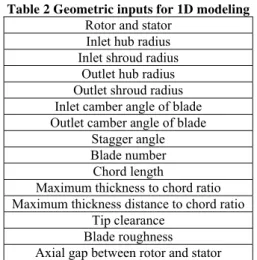
Two types of inputs must be defined for one-dimensional modeling: flow properties and compressor geometry. The entry requirements for design and off-design conditions are not the same. Not only mass flow rate isn’t defined as an input for design condition but also with regard to inlet flow angle, which is calculated with design condition correlation, design mass flow rate is calculated. On the other hand, for off-design, inlet mass flow is defined as an input. Information required as input for design and off-design conditions are presented in Table 1 and Table 2, respectively.

Table 1 Flow inputs for 1D modeling

design Off-design Rotor inlet total

temperature

Rotor inlet total temperature

Rotor inlet total pressure Rotor inlet total pressure Absolute velocity angle

at rotor inlet

Absolute velocity angle at rotor inlet Rotor rotational speed Rotor rotational speed

Mass flow rate

Table 2 Geometric inputs for 1D modeling Rotor and stator

Inlet hub radius Inlet shroud radius

Outlet hub radius Outlet shroud radius Inlet camber angle of blade Outlet camber angle of blade

Stagger angle Blade number Chord length

Maximum thickness to chord ratio Maximum thickness distance to chord ratio

Tip clearance Blade roughness Axial gap between rotor and stator

To predict the performance of the compressor and obtain its characteristic curves, it is necessary to calculate compressor performances at design and off-design points.

2.3

Design Condition

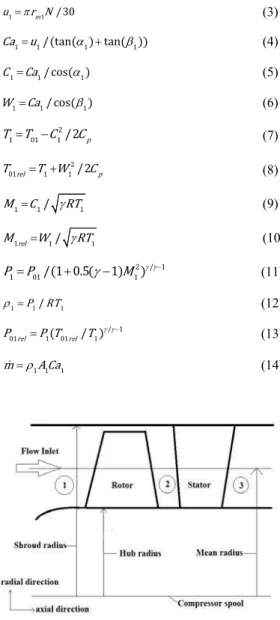
Figure 1 shows schematic of the axial compressor and some geometric parameters. Stations 1, 2 and 3 represent rotor inlet, rotor outlet and stator outlet respectively.

compressor such as inlet and outlet angle of camber line and maximum thickness to chord ratio, it is possible to compute design incidence and deviation angles using Eqs. (1) and (2).



 

* *

, sh t i

i K K i m (1)

 



* *   ,

sh t

K K m (2)

Given the inlet stagnation pressure and temperature, the rotor rotational speed and angles of velocity triangle at rotor inlet, design parameters can be calculated according to Eqs. (3) to (14) “Peyvan (2013).

  m /

u r N (3)

 

 / tan tan

Ca u (4)



 /cos

C Ca (5)



 /cos

W Ca (6)

  / _p

T T C C (7)

  _/

rel p

T T W C (8)



 /

M C RT (9)



 /

rel

M W RT (10)

 

 

 _/  _.  /

P P M (11)

 _{P RT/} (12)

  

 _/ /

rel rel

P P T T (13)

  

m A Ca (14)

Fig. 1. Schematic of meridional view of compressor geometry with three measurement

stations.

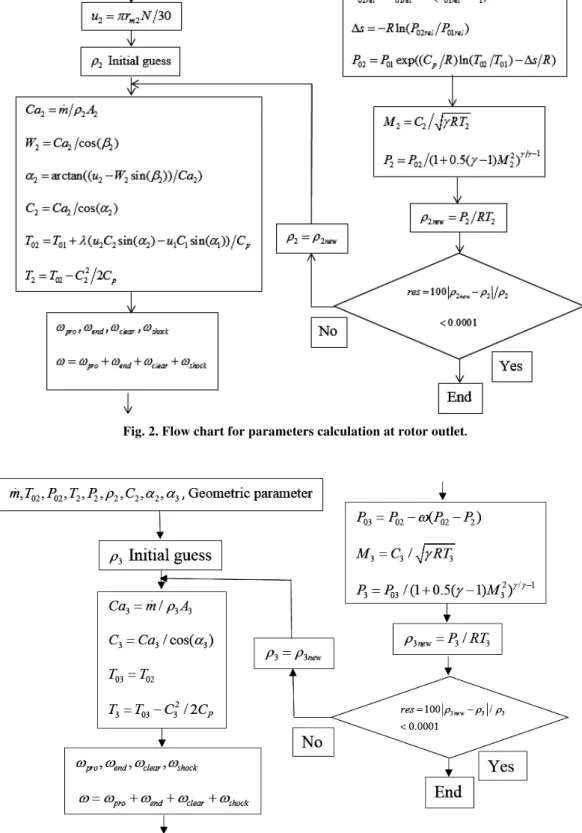
Therefore, the mass flow rate at the inlet of the rotor for design condition is obtained and calculated parameter at rotor inlet set as input to rotor outlet algorithm which is shown in Fig. 2.

After obtaining the unknown parameters at the rotor exit, it is assumed that the flow approaches the stator with design incidence angle. Velocity,

stagnation temperature and pressure at stator inlet are considered the same as calculated at rotor exit. With these assumptions it is possible to compute all parameters at stator inlet. The next step is obtaining unknowns at stator exit by algorithm in Fig. 3.

The outcome of design condition computations is to calculate profile loss coefficients in design condition for rotor and stator rows.

2.4

Off-design Condition

After determination of design profile loss coefficients, it is affordable to obtain profile loss coefficients in off design condition. The coefficient can be obtain through Eqs. (15) and (16). Mass flow rate is the code input for off-design condition. Consequently, for one stage of axial compressor, all the unknown quantities for off design condition in the rotor inlet, rotor exit and stator exit are calculated.

To obtain the off-design loss coefficients a dimensionless parameter for incidence angle is defined as follow “Aungier (2003):

  * _/  *  * ps

i i i i i i

(15)

  * _/ *  *

ns

i i i i i i (16)

ps

i and i_nsare related to incidence angle of positive and negative stall and iis the design incidence angle that is used in correlations represented by Herig Aungier (2003). Herig presented approximate relationships to calculate positive and negative stall incidence angle for NACA 65 series.

   _{ }       _  _ _{ }     . * . ns ns

i i (17)

 _            * _{. .} . . ps ps

i i (18)

Finally off-design loss coefficients are obtained, as follows:

  *_[  _]

shock

   (19)

  *_[   _]

shock

   (20)

*_{[2 2( 1)]}

shock

    

  (21)

First, calculation is performed at the rotor inlet station, based on Fig. 4 algorithm. Thereafter; other unknowns are determined through Eqs. (22) to (27):

(22) 

 _{m off/}

u r N

(23)

 arctan u C sin / cosC 

(24)

 

 cos /cos

W C

(25)



 _/ rel

M W RT

(26)

  /

rel p

T T W C

Fig. 2. Flow chart for parameters calculation at rotor outlet.

Fig. 3. Flow chart for parameters calculation at stator outlet.

 

 _/ /

rel rel

P P T T

₍₂₇₎

The algorithm used for calculating design condition is also applied for off design condition at rotor and

Aungier (2003). Johnson and Bullak (1965) presented a model to calculate variation of deviation angle at design point. After a lot of experiments and corrections they succeeded to obtain a correlation which predicts linear variation of deviation angle based on incidence angle, Eq. (28). According to linear variation of deviation angle with incidence angle and the correction that was made by Pullard and Gastello, considering the effect of axial velocity variation, the deviation angle for off design condition is calculated with Eq. (29).

(28)

 _{   }

  _{ }

  

_  _{ }

 

*

.

. / / exp .

i

(29)



  _ _    

 

*

* * _/

a a

i i W W

i

3.

S

TALL

A

ND

S

URGE

Despite the complexity of the surge phenomeana there are methods that can be used to determine the surge criteria. Aungier (2003) defined a parameter named equal velocity ratio:

(30) 

  rel RE

rel

P P

W

P P

Based on Renao investigations on regular two dimensional diffusers, Aungier (2003) determined stall criteria according to the following equation.

(31)



 







  

 



 

 _{ }

max max

.

. / / . /

. / sin / cos

RE

t c t c

W

Comparing the results of Eq. (31) with the experimental results led to the relationship suitable for diffusion coefficient over 2.2 as Eq. (32) (Aungier 2003).

(32)







 







  

  _{ }

 

 



 

 _{ }

.

max max

.

. / . / / . /

. / sin / cos

eq RE

D t c t c

W

Eq. (32) is valid if relation (33) is satisfied.

(33)

_{/ sin / cos}_   _{ .}

4.

T

HREE

D

IMENSIONAL

M

ODELING

Application of numerical methods for turbomachinery simulation has started since 1940. In fact, these methods have been formulated before digital computers advent. First, streamline curvature was presented by Wu which can be considered as a primary numerical method for turbomachinery and its concept has been used wildly till 1980 when CFD methods were practically applicable Denton and Dawes (1998).

Full three dimensional CFD method considers geometric details such as sweep angle, lean angle and wall profile of axial compressor which results in detailed investigation of flow field. In this study CFD method was used to predict the

performance of a compressor with a specific geometry.

Fig. 4 Flow chart for parameters calculation at rotor inlet for off-design condition.

4.1 Solving Problem with

Three-Dimensional Method

In this research, flow field of a single stage axial compressor of the gas turbine in the laboratory is solved by 3D modeling. In three dimensional modeling the equations of conservation of mass, momentum and energy coupled with ideal gas equation and k-epsilon turbulence model are solved simultaneously to achieve flow field solution Nili-Ahmadabadi et al. (2014).

4.2 Grid Construction

Because of symmetry of flow field it is sufficient to just take a rotor blade and a stator blade into account with definition of proper boundary condition which results in dramatically reducing solving time. Fig. 5 shows the flow field around a rotor blade with boundary conditions.

Flow fields in the rotor and stator are meshed using structured grid (Figs. 6 to 8). The topology of mesh is H/J/C/L. The ratio of number of nodes of rotor domain to stator domain is 60 to 40. The grid independency was performed based on the results which resulted in 500,000 nodes are enough for rotor and stator domains overall in order to obtain an acceptable result.

4.3 Problem Setup

outlet boundary, periodic boundaries 1 and 2, and interface at tip clearance. The air flow passing through the domain is considered as an ideal gas. The energy turbulence model is chosen to be k-epsilon. Types of boundary conditions are very important to complete the problem definition. At inlet (station 1) total temperature and total pressure and flow direction are defined. At stator outlet the amount of output mass flow rate is specified. Three types of interfaces are defined: a) the interface between rotor domain outflow surface and stator inflow surface, b) periodic interface at both sides of rotor and stator domain, and finally, c) the interface at rotor tip clearance which connects pressure side and suction side of the blade tip, see Fig. 8. Moreover, the rotational speed of the rotor is defined.

Fig. 5. Flow field and boundaries.

Fig. 6. Mean surface of rotor (upper) and stator (lower) grid.

5.

E

XPERIMENTAL

S

TUDY

At Sharif University Gas Turbine Laboratory, a small gas turbine engine, equipped in an experimental test bed, see Fig. 9. The gas turbine engine includes a single stage axial compressor which is investigated in this study.

Fig. 7. Rotor blade and the middle control layer.

Fig. 8. Rotor and stator blades, left and right sides respectively.

Fig. 9. Test setup.

5.1 Measurement and Calibration System

There are twelve measuring stations installed on the engine in axial direction, those related to this research are as follows:

1. Inlet of bell mouth, 2. Rotor inlet of axial compressor, 3. Rotor exit, 4. Exit of axial compressor.

5.1.1 Measurement System

A. Pressures: all static pressures are measured using four static pressure taps equally spaced around the circumference of the duct, and joined together and connected to a strain gauge pressure transducer, to give an average static pressure. The total pressures are measured using Pitot tubes connected to the strain gauge pressure transducers.

B. Temperatures: Temperatures are measured using J type thermocouples. The maximum error of the temperature measurement system is about 0.25 0_C

Pourfarzaneh (2010). All thermocouples are connected to the computer data acquisition system by Adams cards Asgarshamsi et al. (2014).

C. Air mass flow rate: The compressor air mass flow rate is measured using a bell mouth entry flow meter. The mass flow calculation is based on pressure drop measurement across the bell mouth throat and ambient temperature and pressure measurements.

D. Rotational speed: The compressor rotational speed is measured using a magnetic pick-up, which counts shaft revolution per second.

5.1.2 Calibration

For calibration of the pressure gauges 2 meters long manometer filled with mercury is used. It is accomplished by measuring different values of pressures by data acquisition system as well as manometers. Thereafter, by a curve fitting the test points with minimum error, the calibration curve is obtained Pourfarzaneh (2010).

In order to calibrate J type thermocouples, some equilibrium temperatures such as ice-water mixture temperature are used. An accurate RTD thermometer is used as well.

5.2 Test Method

The compressed air is blown into the turbine blades and consequently engine speed rises to ignition speed. Then the fuel is injected and the ignition system ignites the mixture of air-fuel and finally. Gradually engine accelerates to higher speeds, which at several steady state conditions, the Automated Data acquisition system records all data every second. All the data obtained from the sensors are calibrated with calibration curves achieved from regression of calibration data points.

5.3 Experimental Results

At this section the axial compressor performances are presented. Fig. 10 shows the running line of pressure ratio versus mass parameter, of the axial compressor from start condition to nominal speed of engine. The trend of the curve is acceptable in comparison with typical one Mattingly and von Ohain (1996). According to this curve, pressure ratio increases as mass parameter and speed.

In Fig. 11, the compressor pressure ratio changes versus speed parameter are shown. In this figure speed parameter increases from idle to rated speed, while pressure ratio the increases from 1.05 to 1.402. With increasing rotational speed, linear speed of the blade increases, therefore output

enthalpy of the compressor increases which causes more pressure augmentation. In Fig. 12, the compressor isentropic efficiency is plotted versus the mass parameter.

Fig. 10. Stagnation Pressure ratio versus mass parameter Mpm kg s( / ) T k0( ) /P bar0( )

(experimental results).

Fig. 11. Stagnation Pressure ratio versus speed parameter NN rpm( ) / T k₀( ) (experimental

results).

Fig. 12. Isentropic efficiency versus mass parameter (experimental results).

5.4 Errors and Uncertainty of Experimental

Results

To calculate the overall uncertainty caused by the combined effects of uncertainties in various variables, the following general equation is introduced Nakra and Chaudhry (2004).

(34)

 _{, ,..., ,...,i n}

y f x x x x

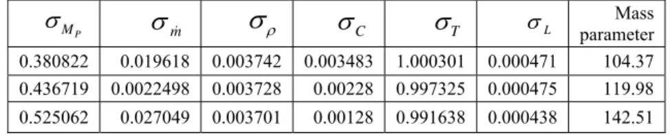
Table 3 Uncertainty values for three values of mass parameter Mass parameter L



T



C







m



_ P M



104.37 0.000471 1.000301 0.003483 0.003742 0.019618 0.380822 119.98 0.000475 0.997325 0.00228 0.003728 0.0022498 0.436719 142.51 0.000438 0.991638 0.00128 0.003701 0.027049 0.525062

the combined effects of different variables can be written as: (35)

 

    _{ }     _ _ _{ }   



 / n I xi i i y x

The term_Iis general uncertainty for y parameter

and the term_xiis uncertainty relating to measured

quantityx_i.

For example, the stagnation pressure ratio uncertainty is obtained by Eq. (36).

(36)



 





  _Pr   

Pr P Pr P /P P /P

P

Experimental results which are extracted from the data that is captured from three measuring stations of gas turbine engine are used for comparison with theoretical results and uncertainty analysis is performed on the data captured at these stations. The values of uncertainties for mass parameter, total pressure ratio and isentropic efficiency are shown in Table 3. According to the obtained values of the uncertainty it can be concluded that the sensors are suitable to be used in the test. As an example for mass parameter of 104.37, uncertainties of mass parameter, pressure ratio, and isentropic efficiency are 0.4, 0.15 and 3 percent respectively.

Table 4 Uncertainty values of efficiency and pressure ratio for values of mass parameter Mass parameter Pr  Tr    104.37 0.001737 0.004952 0.04635 119.98 0.001798 0.00496 0.04336 142.51 0.001866 0.005162 0.033206

6.

O

NE

D

IMENSIONAL

M

ODELING

R

ESULTS

Axial compressor maps are shown in Figs 13 and 14. In these diagrams stagnation pressure ratio and efficiency changes versus mass parameter are plotted in four different rotational speeds. Also surge line of the compressor is plotted. Stall condition is defined according to Eqs. (31) and (32) for rotor and stator rows. If parameter W_REfor rotor row or stator row is less than the value defined by Eq. (32), stall condition occurs. As the rotational speed increases, more pressure ratio is obtained. For

a given rotational speed the curve of pressure ratio versus mass parameter has a negative slope. The curve to the left side and right side is limiting to choking and surge conditions respectively. With a slight increase in mass parameter near choking condition, pressure drop increases sharply resulting the declination of pressure ratio. It is observed that the compressor maximum pressure ratio near surge condition for design rotational speed is 1.432. Surge line is ascending which is the same as those are in the literature.

In order to investigate flow angles, the compressor blade characteristics are briefly presented in Table 5.

Table 5 Compressor blade angles

Inlet camber angle Outlet camber angle Stagger angle

Rotor 51.28o _23.49o _39.9o

Stator 38.28o ₀o _12.06o

There are several performance points which were modeled through 1D modeling so that it is impossible to investigate their velocity triangles. However, the velocity triangles are delineated for three mass flow rate amount at design speed which are shown in Fig. 16.

Fig. 13. Single stage of axial compressor characteristic curve of pressure ratio versus

mass parameter through 1 D modeling.

According to Fig. 14 at a specific mass parameter, isentropic efficiency increases with rotational speed. Similar to pressure ratio graph, efficiency curves are limiting to choking condition with minimum magnitude at right side and surge condition at left side.

mass parameter near the surge condition.

Fig. 14. Single stage of axial compressor characteristic curve of isentropic efficiency

through 1 D modeling.

Fig. 15. Single stage of axial compressor characteristic curve of required power through 1

D modeling.

7.

T

HREE

D

IMENSIONAL

M

ODELING

R

ESULTS

Numerical solution results change considerably with grid size up to a certain amount. Therefore, it is necessary to increase the number of grid to a point which the results don’t change. For 80 percent of design speed and 125.05 mass parameter, flow field is solved with different grid numbers. The compressor pressure ratio and efficiency results are used for grid independency check. It is shown that by increasing the number of grids from 500,000 to 1000,000, pressure ratio and efficiency change about 0.009 and 0.03 percent respectively. Therefore, in order to reduce the computational time with acceptable accuracy, the number of grid points is chosen to be 500,000.

To obtain the characteristic curves of the compressor using three-dimensional method, three rotational speeds the same as one dimensional modeling are selected and flow field is solved for various mass flow rates ranging from surge to choking conditions.

Figures 17 and 18 have similar trend to one dimensional modeling results. The total number of grid is the same for all rotational speeds. For lower rotational speeds the accuracy of solution increases. For a fixed geometry, with increase of speed, time scale reduces so for acceptable error, element size has to be reduced Löhner (2008). In a particular speed, for mass flow rates close to surge condition,

residuals are changed oscillatory and the convergence rate becomes lower. Away from the surge condition and at midpoints, convergence rate increases and residuals do not oscillate. Near choking condition, if mass flow rate wouldn’t be chosen in the proper range, then solution diverges.

8.

C

OMPARISON

O

F

1-

D

A

ND

3-

D

M

ODELING

R

ESULTS

W

ITH

E

XPERIMENTAL

R

ESULTS

Experimental results are averaged on running line of the gas turbine engine resulting a single point for every rotational speed. Therefore, from experimental results all main parameters including, rotational speed, mass flow rate, pressure ratio and efficiency are obtained. According to the experimental data in Figs 10 to 12, due to slight changes in engine condition during the test, and massive data captured, there is some scattering in recorded data.

 

Therefore, data for each point are averaged.

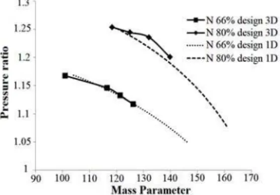
The solid squares shown in Figs 19 and 20 represent experimental results for each speed. It can be seen that the modeling results are in good agreement with experimental results. By connecting these points the compressor running line in gas turbine engine is obtained. Similarly, the efficiency lines are shown in Fig. 20. Maximum differences of 1D results from experimental results are at 66 percent of nominal rotational speed which is 1.2 and 3.8 percent for pressure ratio and efficiency respectively. In Fig. 21, three-dimensional modeling results are compared with the results of one-dimensional modeling in two rotational speeds, which shows very good agreement. Moreover, value of surge mass flow rate obtained by 1D modeling can be used to estimate the more accurate value which can be obtained with 3D modeling in which the surge condition can be specified by the numerical residuals become oscillating Mikhailova et al. (2014). In this sense, the predicted mass parameter for surge condition through 1D and 3D modeling show a slight difference which is about 10 percent of mass parameter predicted by 1D modeling at 80% design rotational speed.

9. C

ONCLUSION

In this study, two methods are used to predict axial compressor performance curves: one and three dimensional modeling.

Mass parameter=141.8 Mass parameter=147.5 Mass parameter=155.35 Fig. 16. Velocity triangles for design rotor speed for three different mass flow rate.

residuals when they become oscillating. Moreover, similarly the maximum mass flow which is possible to pass through the compressor for a specific speed is obtainable through 1D modeling with high slop of efficiency and pressure ratio curves. Furthermore, with estimated value of choking mass flow rate by 1D modeling the mass flow capacity of the compressor is determined by 3D modeling so that mass flow rate for a particular speed can be increased to the point above of which the solution diverges.

Fig. 17. Single stage of axial compressor characteristic curve of pressure ratio through

3-D modeling.

Fig. 18. Single stage of axial compressor characteristic curve of isentropic efficiency

through 3-D modeling.

One significant finding which can be concluded from the comparison of experimental pressure ratio

with 1D modeling is that the compressor works near its surge as the engine reaches its nominal speed.

Comparison between one-dimensional modeling results with experimental results shows good agreements for different rotational speeds. Maximum performance prediction difference for pressure ratio and isentropic efficiency are 2.1 and 3.4 percent respectively. Due to the fact that the experimental results are obtained for a compressor, which is effected by other components of the engine, working inside a gas turbine engine, it can be concluded that the 1D modeling sufficiently predict the performance of a compressor while working in an assembly.

Fig. 19. Comparison of 1-D pressure ratio results with experimental results.

Fig. 21. Comparison of 1-D pressure ratio results with 3-D modeling results.

R

EFERENCES

Asgarshamsi, A., A. H. Benisi, A. Assempour and H. Pourfarzaneh (2014). Multi-objective optimization of lean and sweep angles for stator and rotor blades of an axial turbine. Proceedings of the Institution of Mechanical Engineers, Part G: Journal of Aerospace Engineering, p. 0954410014541080.

Aungier, R. (2003). Axial-Flow Compressors-A Strategy for Aerodynamic Design and Analysis. , ed: New York: ASME Press.

Bullock, R. and I. Johnsen (1965). Aerodynamic Design of Axial Flow Compressors. NASA SP-36.

Denton, J. and W. Dawes (1998). Computational fluid dynamics for turbomachinery design. Proceedings of the Institution of Mechanical Engineers, Part C: Journal of Mechanical Engineering Science 213, 107-124.

Garzon, V. E. and D. L. Darmofal (2003). Impact of geometric variability on axial compressor performance, in ASME Turbo Expo 2003, collocated with the 2003 International Joint Power Generation Conference, 1199-1213.

Horlock, J. H. (1958). Axial Flow Compressors. Florida: Robert E. Krieger publishing CO.

Howell, A. and W. Calvert (1978). A new stage stacking technique for axial-flow compressor performance prediction. Journal of Engineering for Gas Turbines and Power 100, 698-703,

Koch, C. and L. Smith (1976). Loss sources and magnitudes in axial-flow compressors, Journal of Engineering for Gas Turbines and Power 98, 411-424.

Lieblein, S. (1965). Experimental flow in

two-dimensional cascades. NASA Special Publication 36, 183.

Löhner, R. (2008). Applied computational fluid dynamics techniques: an introduction based on finite element methods. John Wiley & Sons.

Madadi, A. and A. H. Benisi (2008). Performance Predicting Modeling of Axial-Flow Compressor at Design and Off-Design Conditions. ASME Turbo Expo 2008: Power for Land, Sea, and Air 317-324.

Mattingly, J. D. and H. von Ohain (1996). Elements of gas turbine propulsion. McGraw-Hill New York.

Mikhailova, A., D. Akhmedzyanov, Y. M. Akhmetov and A. Mikhailov (2014). Joint prediction of aircraft gas turbine engine axial flow compressor off-design performance and surge line based on the expanded method of generalized functions. Russian Aeronautics (Iz VUZ) 57, 291-296.

Nakra, B. and K. Chaudhry (2004). Instrumentation, measurement and analysis. Tata McGraw-Hill Education.

Nili-Ahmadabadi, M., M. Durali and A. Hajilouy (2014). A Novel Aerodynamic Design Method for Centrifugal Compressor Impeller. Journal of Applied Fluid Mechanics 7.

Peyvan, A. (2013). Two-stage axial compressor design software. MSc Theses, Department of Mechanical Engineering, Sharif University of Technology, Tehran.

Pourfarzaneh, H. (2010). Turbojet engine performance modeling and evaluation with experimental test. PHD theses, Department of Mechanical Engineering, Sharif University of Technology, Tehran.

Song, T., T. Kim, J. Kim and S. Ro (2001). Performance prediction of axial flow compressors using stage characteristics and simultaneous calculation of interstage parameters. Proceedings of the Institution of Mechanical Engineers, Part A: Journal of Power and Energy 215, 89-98.

Spina, P. (2002). Gas Turbine performance prediction by using generalized performance curves of compressor and turbine stages. ASME Turbo Expo 2002: Power for Land, Sea, and Air, 1073-1082.