Identification of areas of vote concentration: evidences from Brazil

(1)

R E S E A R C H N O T E

Identiication of Areas of Vote Concentration:

Evidences from Brazil

Glauco Peres da Silva

School of Commerce Foundation Alvares Penteado and Center for

Comparative and International Studies (NECI), Brazil

Andreza Davidian

Center for Metropolitan Studies (CEM) and Center for Comparative

and International Studies (NECI), Brazil

In spite of the recent progress in the discussion on vote regional concentra-tion brought by Avelino et al.(2011), there is still a lack of determination of the districts’ internal areas where candidates obtained their votes. Synthetic concen-tration indices, as the G index, do not allow for evaluation in disaggregated levels, as municipalities, which would be relevant for the verification of the areas of a candidate’s political influence. This paper aims at bridging this gap through the joint utilization of two other indicators, the Location Quotient (LQ) and the Hor-izontal Cluster (HC), that use different measurement units. These indices were applied to the elections of federal representatives in Brazil from 1994 to 2010, and the results were compared to those obtained by Avelino et al.(2011). The appli-cation reaches its aimed result, clearly showing the places where the candidates’ votes are located in the electoral districts.

Keywords: Vote Concentration; proportional elections; G Index; LQ Index; HC Index

Introduction

(2)

However, authors suggest there are deficiencies in the indicators of vote regionalization and suggest a new indicator, the G Index, to measure the vote concentration level for each candidate.

The use of this indicator, however, does not attend to other aspects in the debate, for it does not give information in disaggregated levels of analysis and, thus, does not al-low for the identification of the particular areas where the candidates’ votes are located. These are relevant aspects, for one does not expect either homogeneous or random vote distributions across cities: the votes should reflect the candidates’ efforts to attract sec-tions of the electorate, be it during the campaign or during their mandates. In addition, in order to observe the formation of “reduto”1_{(Hunter and Power, 2007; Zucco, 2008),}

a phenomenon territorially located, indicators of these areas are required. To this effect, we need measures capable of giving disaggregated information on the vote concentration of legislative candidates. The proposed measures are the Location Quotient (LC) and the Horizontal Cluster (HC), taken from indicators used in industrial economics to evaluate the spatial concentration of economic activity. These measures will be applied to federal representatives’ elections from 1994 to 2010 in São Paulo, Brazil.

This paper is divided in three sections. The next section presents the indicators. The following section presents the results when the indicators are applied to cases highlighted in Avelino et al.(2011), in order to show their coherence to the results obtained with the G Index. Last, we present final considerations.

The LQ and HC Indices

As pointed to in Avelino et al.(2011), the traditional indicators of vote concentration are problematic and need to be replaced. The suggested new indicator, the G Index, in-tends to fill the gap, evaluating the spatial concentration of the vote for a particular party or candidate across the whole district. Its formula is given by the expression

G

P

i im m

i

2

∑

(

)

=

−

, (1)

(3)

To this end, they overcome two important difficulties. First, they control for the result of the relative size of each city’s electorates, since in Brazil cities in each district are very heterogeneous as to the size of their electorates. The second advantage is the presentation of an easily interpretable indicator, whose meaning clearly shows the regional distribution of the vote. We believe both indicators operated successfully in this experiment.

To make things clear, we recur to an analogy: assume that each candidate’s vote was previously established in an hypothetical ballot box where voters would randomly take a ballot in order to deposit it in the official ballot box. In this imaginary situation, we would expect to find for each candidate a larger number of votes in cities with the larger number of voters. In other words, the expected spatial vote distribution would be random relative to municipalities, implying that an eventual vote concentration would be a strict function of the number of voters in each city; at the same time, it would be homogeneous relative to the number of voters in each municipality, for there would not be particular interests altering the result. The resulting regional distribution would be due to chance and the representative would be elected according to the total of votes obtained, regardless of their spatial distribution. As we know, this is not what happens. Candidates campaign in specific areas, even when this does not result in concentrated votes (Avelino et al., 2011). But the identification of the places of interest for each candidate may be determined, if we control for the number of voters in each municipality.

In order to overcome this difficulty, we first suggest the utilization of the Location Quotient (LQ), as utilized by Bendavid-Val (1991). Briefly, the LQ may be defined as a measure comparing the proportion of jobs in an activity sector in a regional level to that that would be expected due to the participation of that region in the total work force in the larger area of analysis, be it state or nation. This index shows the relative importance of each region in the sector of the economy under scrutiny, determining if there are work places above what would be expected for that city’s size. Thus, an adaptation for electoral results is

LQ

V

im im i m

=

, (2)

where V_im is the total of votes cast for candidate i in the municipality m,

V

m im i

∑

=

,

V

i im m

∑

=

and

V

im

i m

∑

=

. For the computation of the concentration in each municipali-ty,2_{LQ is a simple measure, for it allows for direct inference of the vote proportion cast for}

(4)

given the total vote cast for the candidate; if it equals 2, the candidate had obtained twice as much as was to be expected, and so on. That information allows for the comparison of the vote obtained per municipality in a homogeneous distribution.

From the LQ, Figleton et al. (2005) propose an adaptation to treat the information on concentration, keeping the original unit with a new index, the Horizontal Cluster (HC). Assume that is the amount of votes that would equal the LQ observed for a candidate in a given municipality to 1. The HC would be equal to

HC

VV

V

(

LQ

1).

i m

=

−

. In other words, if, when LQ equals 1, we have

V

VV

V

im

i m

*

=

_{, then we may say that}

HC

VV

V

(

LQ

1).

i m

=

−

Thus, HC will be larger than zero when LQ is larger than 1, indicating the quantity of votes the candidate obtained above what would be expected in a strictly homogeneous vote distribution. On the other hand, HC would be negative when LQ is smaller than 1, showing exactly how many more votes the candidate would need to reach the homoge-neous distribution. Such an index has an even simpler interpretation than LQ, that is, the number of votes above (or below) the homogeneous distribution. A HC equal to 500 in-dicates thus that the candidate got 500 votes above what would predict the homogeneous distribution. If, on the one hand, LQ gives information that controls for that difference relative to the population in each place, HC informs the size of that difference in number of votes. Both indices allow for an understanding of the vote concentration phenomenon.

Application to Selected Cases

(5)

I. Antonio Carlos Pannunzio

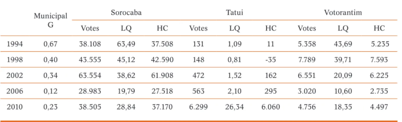
His votes are concentrated around the region of Sorocaba, center-west of São Paulo state, up to the limits with Paraná state. Table 1 shows the evolution of the G Index and of the electoral results, with their respective concentration of his votes in three of the region’s cities.

Table 1. Values computed for Antonio Pannunzio’s votes in the three cities where he got the largest HC in 2010

Municipal G

Sorocaba Tatui Votorantim

Votes LQ HC Votes LQ HC Votes LQ HC

1994 0,67 38.108 63,49 37.508 131 1,09 11 5.358 43,69 5.235

1998 0,40 43.555 45,12 42.590 148 0,81 -35 7.789 39,71 7.593

2002 0,34 63.554 38,62 61.908 472 1,52 162 6.551 20,09 6.225

2006 0,12 28.983 19,79 27.518 563 2,10 295 3.020 10,60 2.735

2010 0,23 38.505 28,84 37.170 6.299 26,34 6.060 4.756 18,35 4.497

Source: Authors elaboration from TSE data

Pannunzio’s vote becomes less concentrated across time. This may be seen in the values of the G Index. The municipal concentration gets systematically lower from 0.67 in 1994 to 0.12 in 2006, with a slight increase to 0.23 in 2010.

(6)

(7)

Figure 1. LQs and HCs maps for Antonio Carlos Pannunzio (PSDB) Source: Own elaboration based on TSE data

This is reflected in the other indicators. In the major town in the region, Sorocaba, with 350,104 voters in 2010, LQ is reduced from 63.5 in 1994 to 19.8 in 2006, with an

increase to 28.8 in 2010. This amounts to say that the candidate obtained in 2010 28.8

times the votes he would have received in a homogeneous spatial distribution, given the

city’s size and the total votes received. The HC index is expressive enough in all elections

considered, highlighting the importance of this municipality for the candidate. In terms of

interpretation, HC shows that of his total 38,505 votes, 37,170 are above what would be

expected under the homogeneous spatial distribution hypothesis. On the other hand, Tatuí presents a large HC only in the 2010 election, with 6,060, a LQ corresponding to 26.3.

With a total number of voters of 62,717 in 2010, its importance for Pannunzio increases

only in the last election. Votorantim presents the same pattern of LQ observed in

Soroca-ba: a decrease from 1994 to 2006, with some increase in 2010. In Figure 1, these variations

are clearly visible. To the left are the figures representing the LQ values and, to the right,

those of HC. We observe the increase of the mass of municipalities with a positive HC, or, alternatively, with the larger LQ, from 1994 to 2006, with some retraction in 2010. In

2006, there are small concentrations in the State’s north, but they disappear in 2010.

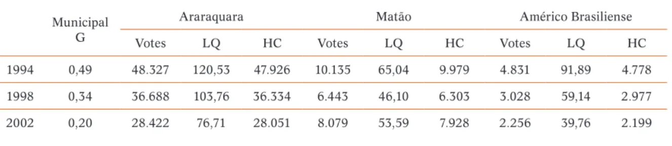
II. Marcelo Fortes Barbieri

Marcelo Barbieri’s votes are situated especially in the Araraquara region, in the

State’s central region. Along the three elections he disputed, his votes concentrate in this

area. Table 2 presents the concentration indices for the 1994 to 2002 elections in which

(8)

Table 2. Values computed for Marcelo Barbieri’s votes in the cities where he got more votes in 2002

Municipal G

Araraquara Matão Américo Brasiliense

1994 0,49 48.327 120,53 47.926 10.135 65,04 9.979 4.831 91,89 4.778

1998 0,34 36.688 103,76 36.334 6.443 46,10 6.303 3.028 59,14 2.977

2002 0,20 28.422 76,71 28.051 8.079 53,59 7.928 2.256 39,76 2.199

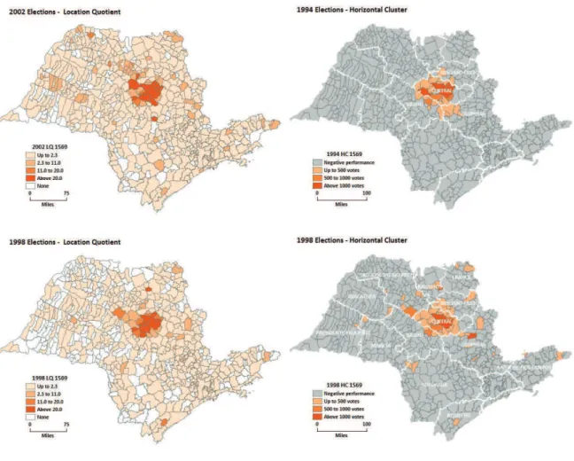
As mentioned in Avelino et al. (2011), the votes are less concentrated across time, what is shown by the values of the municipal Index. This index decreases between elec-tions: in 1994, it is 0.49 and lowers to 0.2 in 2002. In terms of the regional distribution of the votes, as in the previous case, there is a central city, in this case Araraquara, around which the votes are relatively dispersed. There, the LQ values are also reduced across time. In 1994, its value is 120.5, and falls to 76.7 in 2002. A similar profile is that of Américo Brasiliense. The LQ value decreases from 91.9 to 39.8 between 1994 and 2002. On the other hand, in Matão, the LQ falls between 1994 and 1998, but increases again in 2002. This finding allows for the highlighting of the relative importance of the region’s largest city on the concentration indicators, for they vary in the same direction, and at the same time shows that that the values of G and LQ bring about different evaluations. Finally, the values of HC show that Araraquara is decisive for Marcelo Barbieri’s total vote through-out the three elections. The other two cities, even if they present the largest HCs, have a lesser contribution for the spatial vote concentration. That information becomes evident in figure 2.

(9)

Figure 2. LQs and HCs maps for Marcelo Fortes Barbieri (PMDB) Source: Own elaboration based on TSE data

In these maps, the decrease in the concentration of the vote between elections is clearly shown. In 1994, the concentration was clearly defined as shown both by LQ and HC, with few municipalities outside and far of the darker areas of the maps. In subsequent elections, the area becomes less compact and cities appear where the indices are as large as those around Araraquara. That decrease in concentration becomes evident throughout the whole state of São Paulo.

III. Francisco Marcelo Ortiz

(10)

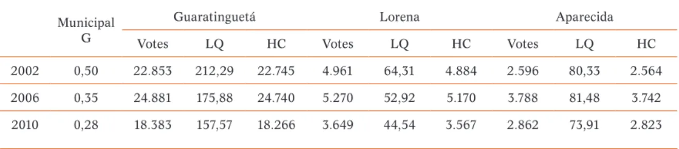
Table 3. Values computed for Marcelo Ortiz’s votes in the cities where he obtained his largest HC in 2010

Municipal G

Guaratinguetá Lorena Aparecida

2002 0,50 22.853 212,29 22.745 4.961 64,31 4.884 2.596 80,33 2.564

2006 0,35 24.881 175,88 24.740 5.270 52,92 5.170 3.788 81,48 3.742

2010 0,28 18.383 157,57 18.266 3.649 44,54 3.567 2.862 73,91 2.823

The G Index presents this decrease in vote concentration, falling from 0.5 in 2002 to 0.28 in 2010. In Guaratinguetá, LQ reaches 212.3 in 2002, falling continuously to still high 157.6 in 2010. In other words, the representative got 157 times the vote he would get under the hypothesis of a homogeneous spatial distribution of the vote. HC also expresses the situation in this municipality, where the total vote was 71,827 in 2010 and Ortiz got 18,266 more than predicted by the homogeneous distribution. Its importance is even more significant when we contrast Guaratinguetá with the other two cities. In Lorena and Apa-recida, while LQ is high enough, HC oscillates around 4 and 3 thousand. This information only emphasize the importance of Guaratinguetá for this representative’s total vote.

(11)

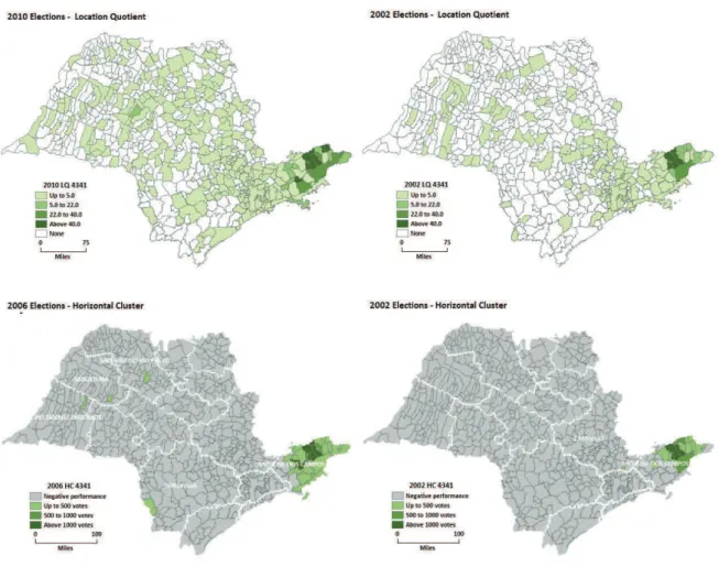
Figure 3. LQs and HCs maps for Francisco Marcelo Ortiz (PV)

Source: Own elaboration based on TSE data

Figure 3 presents the maps for both LQs and HCs for the three elections. As with

the previous cases, we observe the same pattern of evolution over time: there is a clearly

defined concentration in the first election that loses its defined contour in the subsequent

elections. In this case, Ortiz gets his votes in the Vale do Paraíba region in 2002. There

is practically no municipality with a positive HC in that election. But in 2006, cities

be-yond that region present higher values for both LQ and HC and the values for the original

concentrated municipalities are generally lower. In 2010, the process becomes stronger,

pointing to a higher dispersion of the vote in that area.

IV. Telma de Souza

Finally, Telma de Souza repeats the previous cases relative to concentration, with

(12)

concentration from then on. Table 4 presents the information from the indices computed for her vote from 1994 to 2006.

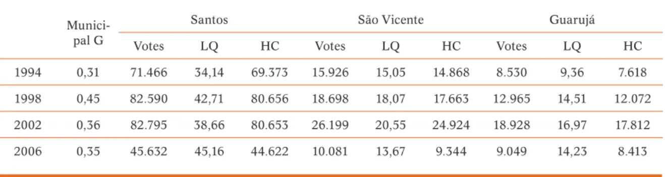
Table 4. Values computed for Telma de Souza’s vote in the cities where she got her largest HC in 2006

Munici-pal G

Santos São Vicente Guarujá

1994 0,31 71.466 34,14 69.373 15.926 15,05 14.868 8.530 9,36 7.618

1998 0,45 82.590 42,71 80.656 18.698 18,07 17.663 12.965 14,51 12.072

2002 0,36 82.795 38,66 80.653 26.199 20,55 24.924 18.928 16,97 17.812

2006 0,35 45.632 45,16 44.622 10.081 13,67 9.344 9.049 14,23 8.413

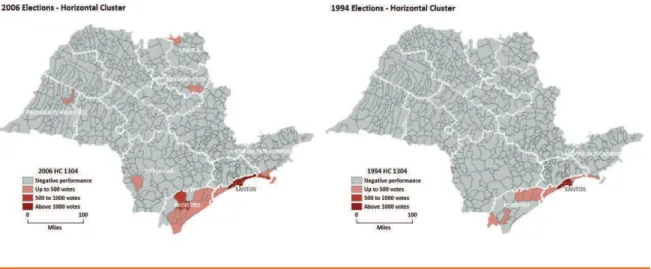
The G Index departs from 0.31, the smallest value in the series, increases in 1998 and declines afterwards down to 0.35 in 2006. As her votes come principally in the Baixada Santista, southern coast of São Paulo, the cities where her votes concentrate are Santos, São Vicente and Guarujá. In the former, LQs vary between 35 and 45, and this was rep-resented by a HC of more than 80 thousand votes in 1998, in other words, around 30% of the total votes in the city and 60% of the vote the candidate obtained in that election. For the other two cities, the values for both LQ and HC are lower, with LQ around 17 in the former and 14 in the later, while HC averages a little bellow 17 thousand in São Vicente and 11.5 thousand in Guarujá. In the graphic representation in the maps, presented in figure 4, the representative’s concentration tendency is very clear.

(13)

(14)

Figure 4. LQs and HCs maps for Telma de Souza (PT) Source: Own elaboration based on TSE data

Last Remarks

The indicators presented, LQ and HC, are capable of showing the areas of vote concentration,

controlling for the size of the population and the representative’s total vote. In this sense,

they are complementary to the G Index presented by Avelino et al.

(2011).

It is worth emphasizing that the variations in all the indices considered, Municipal G, LQ

and HC will not always be in the same direction throughout all cities. The joint movement of

G and LQ may happen when there is a city relatively larger with regard to the others where

the representative has gotten many votes, as happened in the case of Antonio Pannunzio in

Sorocaba. On the other hand, the indicators reveal the spatial dynamics across the territory,

allowing for analyses to be constructed from these results.

Finally, it must be mentioned that, in spite of the data that point to the areas where

representatives get their votes, there is not a necessary association with the construction

of electoral dominance areas. In the cases here presented, it is a well known fact that Iara

Bernardi gets a concentrated vote in the Sorocaba region, as does Pannunzio; that Angela

Guadagnin concentrates her vote in the Vale do Paraíba, as does Marcelo Ortiz; and that

Paulo Mansur shares the Baixada Santista with Telma de Souza. These results call for more

research to discuss the formation of informal electoral districts.

(15)

References

AMES, Barry. (1995a), Electoral Strategy under Open-List Proportional Representation. American Journal of Political Science, vol. 39, nº 2, pp. 406-433.

AMES, Barry. (1995b), Electoral Rules, Constituency Pressures, and Pork Barrel: Bases of Voting in Brazilian Congress. The Journal of Politics, vol. 57, nº 2, pp. 324-343.

AVELINO, George; BIDERMAN, Ciro; SILVA, Glauco Peres da. (2011), A Concentração Eleitoral nas Eleições Paulistas: Medidas e Aplicações. Dados, vol. 54, nº 2, pp. 319-347.

BENDAVID-VAL, Avrom. (1991), Economy Composition Analysis. In: Regional and Local Economic Analysis for Practioners. NY: Praeger, pp. 67-76.

ELLISON, Glenn and GLAESER, Edward L. (1994), Geographic Concentration in U.S. Manufacturing Industries: A Dartboard Approach. NBER Working Paper nº 4.840, <http:// www.nber.org/papers/w4840.pdf?new_window=1> .

FINGLETON, Bernard; IGLIORI, Danilo Camargo; MOORE, Barry C. (2005), Cluster Dynamics: New Evidence and Projections for Computing Services in Great Britain. Journal of Regional Science, vol. 45, nº 2, pp. 283-311.

HUNTER, W. and TIMOTHY, J. P. (2007), Rewarding Lula: Executive Power, Social Policy, and the Brazilian Elections of 2006. Latin American Politics & Society, vol. 49, nº 1, pp.1-30.

MAINWARING, Scott. (1991), Politicians, Parties, and Electoral Systems: Brazil in Comparative Perspective. Comparative Politics, vol. 24, nº 1, pp. 21-43.

ZUCCO, Cesar. (2008), The President´s New Constituency: Lula and the Pragmatic Vote in Brazil´s 2006 Presidential Elections. Journal of Latin American Studies, nº 40, pp. 29-49.

Notes

1 There is no accurate translation for the word ‘reduto’. Ames (1995a: 410) kept the Portuguese use, which would mean, literally, ‘electoral fortress’– a misleading translation in the current stage of the debate, though. Therefore, for our purposes, we will keep using the original term, taking its definition as a particular area of the electoral district from where a candidate receives the highest share of his/her votes.