M
ODELLING AND ANALYSIS OF
FOREST FIRE DATA IN
P
ORTUGAL
-P
ART
II
Giovani L. Silva
CEAUL & DMIST - Universidade Técnica de Lisboa [email protected]
Maria Inês Dias
CIMA & DM - Universidade de Évora [email protected]
In the last decade, forest fires have become a natural disaster in Portugal, causing great forest devastation, leading to both economic and environmental losses and putting at risk populations and the liveli-hoods of the forest itself. In this work, we present Bayesian hierarchi-cal models to analyze spatio-temporal fire data on the proportion of burned area in Portugal, by municipalities and over three decades. Mixture of distributions was employed to model jointly the propor-tion of area burned and the excess of no burned area for early years. For getting estimates of the model parameters, we used Monte Carlo Markov chain methods.
Keywords: Forest fire data, Spatio-temporal modelling, Mixed model, Bayesian analysis.
1
I
NTRODUCTION
According to the National Forestry Authority (Direcção Geral dos Recursos
Florestais), Portugal has the largest number of forest fires among five Mediter-ranean countries (Portugal, Spain, France, Italy and Greece). In order to look for spatio-temporal patterns of fires, we can model the proportion of burned area (Y), which is a (0,1)-restricted continuous variable, assum-ing naturally a beta distribution [4] or Gaussian distribution and a Skew-Normal [2] distributions after a logit transformation, i.e. log(Y /(1−Y )). In addition, we can use Bayesian hierarchical models to take into account spatially correlated random effects[6] and excess zeros in the proportion of burnt area by municipalities and years [1]. Our aim is to present a
spatio-temporal analysis of forest fires in 278 Portuguese municipalities between 1980 and 2006, from a Bayesian perspective and using Monte Carlo Markov chain (MCMC) methods to make inference on the parameters of interest.
2
S
PATIO
-
TEMPORAL MODELING
Let Yi t the proportion of burned area in municipality i and year t, i =
1, . . . , n, t=1, . . . , T. Assume Yi t or log(Yi t/(1−Yi t)) has a probability
distri-bution with meanµi tand varianceσ2. [6] suggest that µi tcan be expressed
by
µi t= α + S0(t) + Si(t) + φi, (1)
where S0(t) can represent a nonlinear temporal effect, Si(t) is the temporal
effect by region i andφi a random effect of the spatial variation associated
with region i. If φi = bi + hi, component hi represents the unstructured
spatial random effect with Gaussian priori distribution, i.e.,
hi ∼ N (0, σh2≡τ
−1
h ), (2)
and bithe spatially correlated random effect with priori distribution, p(bi|τb =
σ−2
b ), chosen in terms of a conditional autoregressive model (CAR) [3], i.e.,
bi | b−i,σ2b∼ N (¯bi,σ2b/mi), (3)
where ¯bi is the mean of the random effects related to the “neighbors” of the
region i, mi the number of adjacent regions to region i andσ2b the variance
component.
Upon the occurrence of zeros, the distribution of the proportion of area burned(Yi tis considered a mixture of distributions with probability function
f(yi t), denoting f1(yi t) = f (yi t| yi t 6= 0), i = 1, . . . , n, t = 1, . . . , T . Define
Vi t as a Bernoulli random variable such that, Vi t = 0, with probability pi t0,
and 1, with probability pi t1 ≡ 1−pi t0, where pi t0 represents the probability
of non-burned area in the region i in the year t. Vi t indicates the existence
of the burnt area in the region i in the year t. Thus,
f(yi t) = f1(yi t)
Vi t(1 − p
i t0)
Vi tp1−Vi t
i t0 . (4)
The probability of no burned area in the region i at time t is modeled as, log p i t0 1− pi t0 = β0+ β1t+ ψi, (5)
whereψi is also a CAR model. We use assigned highly dispersed but proper
priors. In fact, one typically assumes independent normal prior for the re-gression coefficients. For the variance component hyperparameters, one
usually assigns an inverse gamma prior, e.g., σ2∼ I G(r1, s1), σ2b ∼ (r2, s2),
σ2
h∼ I G(r3, s3) and σ2ψ∼ I G(r4, s4) with kernel density given for
x−(r+1)e x p(−s/x), x > 0.
Consequently, we can construct the related joint posteriori distribution and use MCMC methods because the corresponding marginal posteriors are not easy to get explicitly. Notice that these methods are implemented e.g. in WinBUGS [5].
3
F
OREST FIRES DATA ANALYSIS
Based on the models in section 2, we analyze the proportion Yi t of burnt
area due to forest fires in 278 municipalities (mainland Portugal) and over 27 years (1980-2006). Data were collected by Portuguese National Forestry Authority. Three scenarios were considered for the data modeling:
A) Gaussian probability model: l o g i t(Y ) ∼ N(µ, σ2);
B) Skew-normal model: l o g i t(Y ) ∼ SN(µ, σ2,λ), where λ is a shape
parameter;
C) Beta model: Y ∼ Beta(a, b), with E[Y ] = µ, Var(Y ) = µ(1−µ)γ+1 and
γ = a+b.
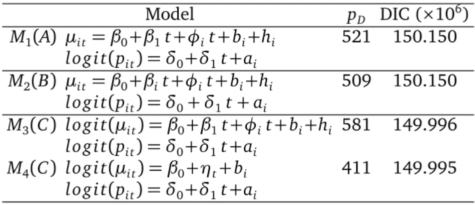
By using MCMC methods via WinBUGS, we used 15,000 iterations for all fitted models, taking every 10th iteration of the simulated sequence, after 5000 iterations of burn-in. The model comparison can be based on the Deviance Information Criterion (DIC), which handles hierarchical Bayesian models of any degree of complexity, and is computed as the sum of two components: the expected posterior deviance (D) and the effective number of parameters (pD), measuring the goodness of fit and complexity of the
model, respectively[7]. It is often expressed as
DI C = 2 D(θ ) − D(θ ), (6)
where D(θ ) and θ denote the posterior mean of the deviance and the model parameter vector θ , respectively. Though we rely principally on this mea-sure for assessing models in our application, the other meamea-sures are also computed for comparison. In table 1, one can be observed some fitted mod-els and, based on (6), the selected model is model M4. Note that S0(t) = ηt,
Model pD DIC (×106) M1(A) µi t = β0+β1t+φi t+bi+hi 521 150.150 l o g i t(pi t) = δ0+δ1t+ai M2(B) µi t = β0+βit+φit+bi+hi 509 150.150 l o g i t(pi t) = δ0+ δ1t+ ai M3(C) logit(µi t) = β0+β1t+φi t+bi+hi 581 149.996 l o g i t(pi t) = δ0+δ1t+ai M4(C) logit(µi t) = β0+ηt+bi 411 149.995 l o g i t(pi t) = δ0+δ1t+ai
Table 1: Model selection based on DIC.
For selected model (M4), the posteriori mean, standard deviation (SD)
and 95% highest posterior density (HPD) credible intervals (CI) of some pa-rameters of interest are in table 2. Based on model M4, the spatio-temporal
risks of burned area, defined here by exp(ηt+ bi) for municipality i, were
used to produce maps in 1985, 1994 and 2001 in figure 1. Parameter Mean SD 95% HPD CI δ1 -0.169 0.007 (-0.183, -0.156) γ 24.82 0.449 (24.02, 25.69) σ2 b 0.334 0.051 (0.237, 0.437) σ2 η 3.357 0.508 (2.424, 4.379) σ2 a 0.194 0.060 (0.098, 0.313) pi t0 0.143 0.003 (0.137, 0.150)
Table 2: Estimates of the model parameters (M4).
4
C
ONCLUDING REMARKS
The spatio-temporal analysis of the burned area proportion in 278 munici-palities of mainland Portugal between 1980 and 2006 reveals an increasing trend in the proportion of burned area, whereas the number of municipal-ities without burned area trend to decrease. The space-time models stud-ied here have smoothed estimates used in the production of maps that are useful in the interpretation of spatio-temporal data. This analysis of the Portuguese forest fires may isolate trends in small areas of administrative knowledge for promoting an appropriate policy interventions to reduce that national catastrophe.
Figure 1: Spatio-temporal risks in 1985 (left), 1994 (middle) and 2001 (right).
A
CKNOWLEDGEMENTS
This paper was partially supported by Pest-OE/MAT/UI0006/2011.
R
EFERENCES
[1] Amaral-Turkman M.A., Turkman K.F., Le Page, Y. and Pereira J.M. (2011) Hierarchical space-time models for fire ignition and percent-age of land burned by wildfires, Environmental and Ecological
Statis-tics, 18, 601-617.
[2] Azzalini, A. and Dalla Valle, A. (1996). The multivariate skew-normal distribution, Biometrika, 83, 715-726.
[3] Besag, J., York, J.C. and Mollié, A. (1991). Bayesian image restora-tion, with two applications in spatial statistics (with discussion),
An-nals of the Institute of Statistical Mathematics, 43, 1-59.
[4] Ferrari, S.L.P. and Cribari-Neto, F. (2004). Beta regression for model-ing rates and proportions, Journal of Applied Statistics, 31, 799-815. [5] Lunn, D.J., Thomas, A., Best, N. and Spiegelhalter, D. (2000).
extensibility, Statistics and Computing, 10, 325-337 (http://www.mrc-bsu.cam.ac.uk/bugs/).
[6] Silva, G.L., Dean, C.B., Niyonsenga, T. and Vanasse, A. (2008). Hi-erarchical Bayesian spatiotemporal analysis of revascularization odds using smoothing splines, Statistics in Medicine, 27, 2381-2401. [7] Spiegelhalter, D.J., Best, N.G., Carlin, B.P. and van der Linde, A.
(2002). Bayesian measures of model complexity and fit, Journal of