doi: 10.1590/0101-7438.2015.035.01.0073
ARTIFICIAL NEURAL NETWORK AND WAVELET DECOMPOSITION IN THE FORECAST OF GLOBAL HORIZONTAL SOLAR RADIATION
Luiz Albino Teixeira J´unior
1, Rafael Morais de Souza
2*,
Mois´es Lima de Menezes
3, Keila Mara Cassiano
3,
Jos´e Francisco Moreira Pessanha
4and Reinaldo Castro Souza
5Received January 23, 2013 / Accepted May 7, 2014
ABSTRACT.This paper proposes a method (denoted by WD-ANN) that combines the Artificial Neural Networks (ANN) and the Wavelet Decomposition (WD) to generate short-term global horizontal solar ra-diation forecasting, which is an essential information for evaluating the electrical power generated from the conversion of solar energy into electrical energy. The WD-ANN method consists of two basic steps: firstly, it is performed the decomposition of levelpof the time series of interest, generating p+1 wavelet orthonormal components; secondly, thep+1 wavelet orthonormal components (generated in the step 1) are inserted simultaneously into an ANN in order to generate short-term forecasting. The results showed that the proposed method (WD-ANN) improved substantially the performance over the (traditional) ANN method.
Keywords: wavelet decomposition, artificial neural networks, forecasts.
1 INTRODUCTION
The conversion of solar energy into electrical energy is one of the most promising alternatives to generate electricity from clean and renewable way. It can be done through large generating plants connected to the transmission system or by small generation units for the isolated systems.
*Corresponding author.
1Latin American Institute of Technology, Infrastructure and Territory, Federal University of Latin American Integration – UNILA, Foz do Iguac¸u, PR, Brazil. E-mail: [email protected]
2Department of Accounting, Federal University of Minas Gerais – UFMG, Belo Horizonte, MG, Brazil. E-mail: [email protected]
3Department of Statistics, Fluminense Federal University – UFF, Rio de Janeiro, RJ, Brazil. E-mails: moises [email protected]; [email protected]
4Institute of Mathematical and Statistics, State University of Rio de Janeiro – UERJ, Rio de Janeiro, RJ, Brazil. E-mail: [email protected]
The Sun provides the Earth’s atmosphere annually, approximately, 1.5×10¹⁸kWh of energy, but only a fraction of this energy reaches the Earth’s surface, due to the reflection and absorption of sunlight by the atmosphere. One problem of renewable energy, for instance, wind and solar energies is the fact that the production of these sources is dependent on meteorological factors. In the case of solar energy particularly, the alternation of day and night, the seasons, the passage of clouds and rainy periods cause great variability and discontinuities in the production of elec-tricity. Also in this case, there is the necessity to have capable devices of storing energy during the day in order to make it available during the night such as battery banks or salt tanks (Wittmann et al., 2008). Thus, the safe economic integration of alternative sources in the operation of the electric system depends on accurate predictions of energy production, so that operators can make decisions about the maintenance and dispatch of generating units that feed the system.
Among the techniques employed in solar radiation forecasting, it can be highlighted the ARIMA (Perdomo et al., 2010), the artificial neural networks (ANN) (Zervas et al., 2008; Yona & Senjyu, 2009; Deng et al., 2010; Yanling et al., 2012; Zhang & Behera, 2012), the neuro-fuzzy systems (ANFIS), the Kalman Filter (Chaabene & Ammar, 2008) and the different ways of combining orthonormal wavelet bases and ANN (Cao et al., 2009; Zhou et al., 2011).
Wavelets have been used in the time series literature combined with other types of predictive models and resulting in significant gains in terms of modeling. In this context, the wavelet theory consists in an auxiliary pre-processing procedure of the series in question, which can be accomplished generally in two ways: by decomposition or by noise shrinkage of the time series to be modeled. There are several studies that highlighted the gains from the combinations of decomposition and/or wavelet shrinkage and neural networks, among which it is possible to mention: Krishna et al. (2011), who applied the combination to model river flow; Liu et al. (2010), Catal˜ao et al. (2011) and Teixeira Junior et al. (2011), who modeled wind time series; Teixeira Junior et al. (2012), who worked with series of solar radiation; and Minu et al. (2010), who studied time series of number of terrorist attacks in the world.
In this article, it is proposed a method (denoted by WD-ANN) to generate short-term forecasts of global horizontal solar radiation, which is an essential information for evaluating the electrical power generated from the conversion of solar energy into electrical energy. In summary, the forecasts of WD-ANN method are obtained from the combined use of an ANN and a wavelet decomposition of p level. More specifically, it starts with the wavelet decomposition level p (Faria et al., 2009; Teixeira Junior et al., 2011; Perdomo et al., 2010) of the time series of global horizontal solar radiation, generatingp+1 orthonormal wavelet components. Then these wavelet components are used as the set of input patterns of an ANN, which is structured to generate short-term forecasts of global horizontal solar radiation.
In the computational experiments, it was used the hourly time series of average global hori-zontal solar radiation (W/m2) obtained from the Solarimetric stations of Sonda Project INPE/ CPTEC6 (Pereira et al., 2006), for 10 locations in Brazil: Bras´ılia, Caic´o, Campo Grande,
Cuiab´a, Florian´opolis, Joinville, Natal, Palmas, Petrolina and S˜ao Martinho. Only for Cuiab´a the analysis is reported with minor details. All time series cover exactly a period of one year, but a different year in each location.
The paper is organized into six sections. In Sections 2 and 3, there are introduced theoretical aspects of Wavelet Theory and Neural Networks, respectively. The WD-ANN method is detailed in Section 4. The computational experiments and its main results are presented in Section 5. In Section 6, there are the conclusions of the research.
2 WAVELET THEORY
2.1 Hilbert Space, Orthonormal Basis and Fourier Series
According to Kubrusly (2001), a Hilbert space H is any linear space equipped with an inner product and complete. The collectionl2of all infinite sequences of complex numbers quadrat-ically summable (in other words,l2 := {f : Z→ C:
t∈Z|f(t)|2 <∞}), provided with an
inner product<;>(that is,<;>:l2→C), or, simply, the pair (l2, <;>), is a particular case of Hilbert space (Kubrusly, 2001). According to Kubrusly & Levan (2002), a subspace{hn}n→Zof
a Hilbert space H is a orthonormal basis of H if, and only if, satisfies the axioms (i), (ii) and (iii).
(i) orthogonality:h′n,hm =0, whenevern′=m, wheren′,m∈Z;
(ii) normality:||h′n|| =1, wheren′∈Z;
(iii) completeness:x,h′n =0 if, and only if,x=0.
According to Theorem of Fourier series (Kubrusly, 2001), if the subset{hn}n∈Zis an
orthonor-mal basis, then the identity in (1) is a single expansionxof H in terms of the orthonormal basis
{hn}n∈Z. The expansion in (1) is called a Fourier Series.
x=
n∈Z x,hn
||hn||
hn. (1)
2.2 Wavelet Function
Consider a Hilbert space(l2, <;>). One elementω(.)∈l2– with an inner product<;>:l2→
C– is called wavelet function if, and only if, the functionsωm,n(.):=2m/2ω(2m(.)−n), where
n,m ∈ Z, form an orthonormal basis for the Hilbert space(l2, <;>). According to (Levan & Kubrusly, 2003), any function f(.)in(l2, <;>)admits the Fourier series expansion in terms of an orthonormal basis wavelet{ωm,n(.)}(m,n)∈Z×Zofl2, as in (2).
f(.)=
m∈Z
n→Z
f(.), ωm,n(.)ωm,n(.) (2)
wheremis called scaling parameter andnis called translation parameter (Ogden, 1997).
closed subspace (Kubrusly, 2001) Wm(ω):=(span{ωm,n(.)}n∈z)−of(l2, <;>)is called details subspace (on scalingm). In turn, the projection of f(.)on (closed) subspace of details Wm(ω), denoted by fWm(ω)(.), is defined by the partial sum showed in (3).
fWm(ω)(.):=
n∈Z
f(.), ωm,n(.)ωm,n(.) (3)
According to Levan & Kubrusly (2003), the projection fWm(ω)(.)can be interpreted as a detail
component of f(.), on scalingm, on(Wm(ω), <;>). As a result, given the identity (1), it follows that f(.)can be interpreted as a sum of all detail components fWm(ω)(.), at all entire scaling m, on closed subspace n∈zWm(ω)
−
, <;>
of(l2, <;>). Tautologically, it follows that
n∈zWm(ω) −
, <;>=(l2, <;>).
On the other hand, one elementφ (.) ∈ l2 – with an inner product<;>: l2 ∈ C– is called wavelet scaling function (or simply scaling function) if, and only if, the functionsφm,n(.) := 2m/2φ (2m(.)−n), wheren,m ∈ Z, are such thatφm′,n′(.), φj,k(.) = 0, wheneverm′ = j and n′ = k, and φm′,n′(.), φj,k(.) = 0 else. According to Mallat (1998), the closed sub-spaceVm(φ):=span{φm,n(.)}n∈Z
−
of(l2, <;>)is called approximation subspace (on scaling m). The projection of f(.)on (closed) subspace of approximationVm(φ)is defined by the sum described in (4).
fVm(φ)(.):=
n∈Z
f(.), φm,n(.)φm,n(.) (4)
According to Mallat (1998), fVm(φ)(.)can be interpreted as an approximation component of f(.),
on scalingm, on subspace(Vm(φ), <;>)de (l2, <;>).
2.3 Wavelet Transform
Wavelet transform on(l2, <;>), is the inner product<;>:l2→Cbetween a functionf(.)∈l2 and a wavelet functionωm,n(.)∈Wm(ω)or a scaling functionφm,n(.)∈Vm(φ), (m,n)∈Z×Z. According to Mallat (1998), the wavelets transforms can be classified and grouped into two distinct sets: detail coefficients, denoted by {dm,n}(m,n)∈Z×Z, and approximation coefficients,
denoted by {am,n}(m,n)∈Z×Z. For each ordered pair (m,n) ∈ Z×Z, it has that the wavelet
transformsdm,nandam,nare defined, respectively, by
dm,n:= f(.), ωm,n(.) =
t∈Z
f(t)ωm,n(t) and
am,n:= f(.), φm,n(.) =
t∈Z
f(t)φm,n(t).
2.4 Wavelet Expansion
According to Levan & Kubrusly (2003), a chain of approximation subspaces {Vm(φ)}m→Z
(a) Vm(φ)⊂Vm+1(φ), ∀m∈Z;
(b) ∩m∈ZVm(φ)= {0};
(c)
∪m∈ZVm(φ)
−
=H;
(d) v∈Vm(φ)⇔Dv∈Vm+1(φ),m∈Z; and
(e)
2m/2φ (2m(.)−n)n∈
Zis an orthonormal basis ofVm(φ),m∈Z.
In Kubrusly & Levan (2002), it is shown that al2space can be orthogonally expanded such as l2 = m∈
zWm(ω)
−
, and in Levan & Kubrusly (2003), it is shown, using the axioms of a wavelet MRA{Vm(φ)}m∈z, that the identityVm0(φ) =
m0−1
−∞ Wm(ω)
−
, for allm0 ∈ Z, is true. Based on the identitiesl2= m∈zWm(ω)−andVm0(φ)= m0−1
−∞ Wm(ω) −
, and on Theorem of Orthogonal Structures (Kubrusly, 2001), it is shown in Kubrusly & Levan (2002) that thel2space can be orthogonally expanded as in (5).
l2=Vm0(φ)+
+∞
m=m0
Wm(ω)
−
(5)
As a result, it follows that f(.)has (a single) orthogonal decomposition on the Hilbert space (l2, <;>), as in (6).
f(.)= fVm
0(φ)(.)+
+∞
m=m0
fWm(ω)(.) (6)
Given the definitions of wavelet components fVm
0(φ)(.)and fWm(ω)(.)and the identities (1) and
(6), it follows that the Fourier series of function f(.), on the Hilbert space (l2, <;>), in terms of the orthonormal basis wavelet{φm0,n(.)}n∈z∪ {ωn,m(.)}(m,n)∈{m}+∞m0 ×z, is given by:
f(.)= n∈z
am0,nφm0,n(.)+
+∞
m=m0
n∈z
dm,nωm,n(.) (7)
where: am,n :=
t∈Z f(t)φm,n(t), dm,n := t∈Z f(t)ωm,n(t), where m0 ≤ m < +∞ andm0∈Z.
3 ARTIFICIAL NEURAL NETWORKS
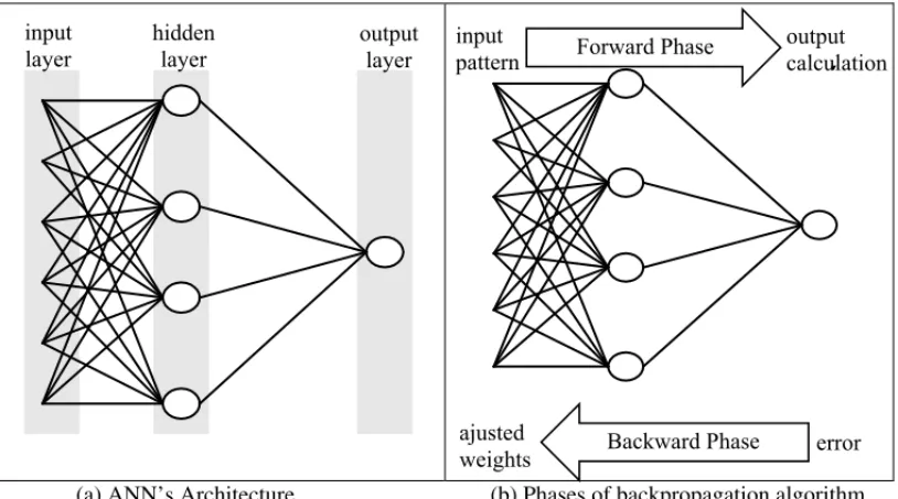
According to Haykin (2001), Artificial Neural Networks (ANN) are distributed parallel systems composed of simple processing units called artificial neurons. They are arranged in one or more layers interconnected by a large number of connections (synapses), which are generally unidirec-tional, and they have weights to balance the inputs received by each neuron. The most common architecture of an ANN is the multilayer perceptron with three layers (input, hidden, and output), as shown in Figure 1(a).
The first layer of the ANN is the input layer, the only one who is exposed to input variables. This layer transmits the values of the input variables to neurons of the hidden layer so that they can extract the relevant features (or patterns) of the input signals and transmit the results to the output layer. The definition of the number of neurons in each layer is performed empirically. The ANN’s training consists of an iterative process to obtain the weights of connections between processing units.
The main training algorithm is named backpropagation, whose weights’ fit occurs through an optimization process of two phases: forward and backward, as shown in Figure 1(b). In the forward phase, it is calculated a response provided by the network for a given input pattern. In the backward phase, the deviation (error) between the desired response (target) and the re-sponse provided by the ANN is used to adjust the weights of the connections.
saída
(a) ANN’s Architecture (b) Phases of backpropagation algorithm
output calculation input
pattern
Backward Phase error ajusted
weights
Forward Phase input
layer
hidden layer
output layer
Figure 1– Multilayer perceptron artificial neural network. (a) ANN’s Architecture; (b) Phases of back-propagation algorithm.
During the neural network training, the various input patterns and their corresponding desired outputs are presented to the ANN, such that the weights of synapses are corrected iteratively by gradient descent algorithm in order to minimize the sum of squared errors (Haykin, 2001).
The time series forecasting through ANN starts by the assembly of the training patterns (in-put/output pairs) that depends on the setting of the window size L of time (to the past values of the series and to the explanatory variables) and the forecast horizonh. In an autoregressive process (linear or nonlinear), for example, the input pattern is formed only by past values of the series itself.
In Figure 2, it is illustrated how is generally constructed the training set for the forecast based on the past four values passed. Note that the training patterns’ construction of the network consists of moving the input and output windows along the entire time series. Thereby, each pair of windows (input/output) serves as a training pattern and must be presented repeatedly until the learning algorithm converges.
time series
time
input network = n past values example: n=4
input window
desired output = values to k steps ahead
example: k=1
output window
Figure 2– Setting of the training set.
4 COMBINATION OF ARTIFICIAL NEURAL NETWORKS
AND WAVELET DECOMPOSITION
The combination of an ANN and wavelet decomposition (WD) may be performed in many dif-ferent ways. For instance, it can be applied the wavelet decomposition in the time series. Then, each resultant series have to be modeled by the traditional ANN, and finally, it should add the series’ forecasts in order to obtain the forecast of the original time series. Another option is to use wavelet functions (normalized in the range[0,1]) as activation functions of neurons of a traditional ANN and to utilize the input of decomposed patterns through WD.
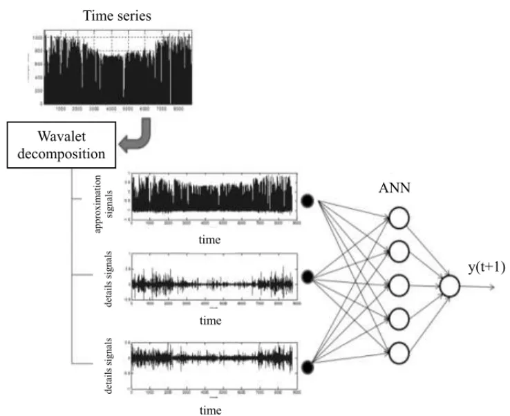
In this article, however, it was chosen a combining method (denoted by WD-ANN), in which the wavelet components of the time series are the input patterns of a feedfoward MLP ANN whose output provides a time series forecast (according to the diagram of Fig. 3). Basically, the proposed approach can be divided into steps (1) [described in Section 4.1] and (2) [described in Section 4.2]:
(1) To make the wavelet decomposition of level p (Reis & Silva, 2004; Lei & Ran, 2008; Teixeira Junior et al., 2011) of a time series f(.); and
Time series
Wavalet decomposition
ANN
y(t+1)
approxim
ation
si
g
nals
details signals
details signals
time
time
time
Figure 3– Combination of wavelet decomposition+ANN.
4.1 Wavelet decomposition of level p
Let f(.)be a time series of (l2, <;>), and{φm0,n(.)}n∈z∪ {ωn,m(.)}(m,n)∈{m}+∞m0 ×zbe a orthonor-mal wavelet basis of Hilbert space (l2, <;>). According to identity (7), the wavelet decomposi-tion of level p(Teixeira Junior et al., 2011) of f(.), where pis a natural number inside interval 1≤ p<∞, is represented by the (approximated) Fourier series described in (8).
f(.)≃≈f(.)= nm0
n=1
am0,nφm0,n(.)+
nm
n=1
m0+(p1)
m=m0
dm,nωm,n(.) (8)
The optimal values of the parameters m0, nm0 and{nm}
m0+(p−1)
m=m0 are such that minimize the
Euclidean metric (Kubrusly, 2001) from the time series f(.)and your approximation ≈
f(.). The wavelets components fVm0(φ)(.) :=
n∈zam0,nφm0,n(.)and fWm(ω)(.) :=
n∈zdm,nωm,n(.) are classified, respectively, as approximation component (atm0scale) and detail component (at
mscale) of time series f(.)of (l2, <;>). Given the expansion (8), it follows that the time series can be expanded orthogonally on (l2, <;>), as in (9).
f(.)≃ fVm
0(φ)(.)+
m0+(p−1)
m=m0
where fVm0(φ)(.) =
fVm0(φ)(t)
t∈Z, for a fixed integerm0, and fWm(ω)(.) =
fWm(ω)(t)
t∈Z,
wheremis an integer inside the intervalm0≤m≤m0+(p−1), beingpthe level of wavelet decomposition.
4.2 Submission of the wavelet components to the ANN Take a feedforward MLP ANN. The set of temporal signals
fVm0(φ)(t)
T
t=1
∪
fWm(ω)(t)
T
t=1
m0+(p−1)
m=m0
arising from p +1 wavelet components of a time series{f(t)}Tt=1 [Section 4.1] are such that constitute the set of input patterns to a feedforward MLP ANN to the training process.
Whereas a window size equal toL past values, the time series forecast (the output of ANN) for eacht′time (in training, validation and test samples) is obtained from the set of input patterns described in (10).
fVm
0(φ)(t)
t′−1
t=t′−L fVm(ω)(t)
t′−′
t=t′−L
m0+p(p−1)
m=m0
(10)
5 COMPUTATIONAL EXPERIMENT
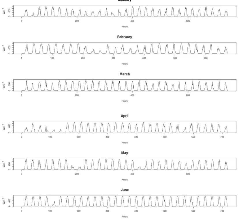
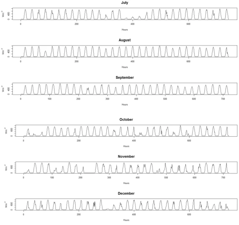
In the computational experiments, it was considered the hourly time series of global horizontal solar radiation during the period from January to December. The representation of the daily profiles of solar radiation at ten different locations for different years is showed in Figure 4.
The sample used in ANN’s training contain 7008 observations of solar radiation, while the fol-lowing 876 observations belong to the validation and the last 876 to test samples. The train-ing of ANN was performed in MATLAB software. In all simulations, the input patterns were normalized by the premnmx transformation and the training algorithm used was Levenberg & Marquardt.
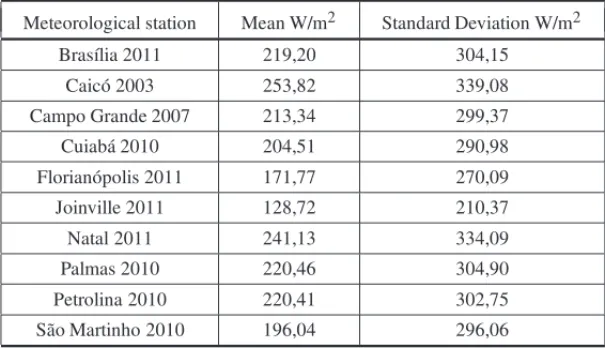
It was chosen the ANN (feedforward MLP) with the best fit to the series of global horizontal solar radiation. The yearly average and standard deviation of the ten series are presented in Table 1. The standard deviation provides a measure of the yearly variability of the global horizontal solar radiation.
In this paper, it is reported the detailed results from Cuiab´a whose radiance time series in each month is illustrated in Figure 5.
For the time series from Cuiab´a, the best identified ANN [Section 5.1] presents the following topological structure: input window size equal to 10; one hidden layer composed of 19 artificial neurons with activation function hyperbolic tangent; and one neuron in the output layer with linear activation function (Haykin, 2001).
Wm
2
Wm
2
Hours Hours
Brasília 2011 Caicó 2003
Brasília 2011
Wm
2
Wm
2
Wm
2
Wm
2
Hours Hours
Hours Hours
Campo Grande 2007 Cuiabá 2010
Florianópolis 2011 Joinville 2011
Florianópolis 2011
Natal 2011 Palmas 2010
Petrolina 2010 São Martinho da Serra 2010
Hours Hours
Hours Hours
Wm
2
Wm
2
Wm
2
Wm
2
Table 1– Mean and standard deviation of the global horizontal solar radiation.
Meteorological station Mean W/m2 Standard Deviation W/m2
Bras´ılia 2011 219,20 304,15
Caic ´o 2003 253,82 339,08
Campo Grande 2007 213,34 299,37
Cuiab´a 2010 204,51 290,98
Florian´opolis 2011 171,77 270,09
Joinville 2011 128,72 210,37
Natal 2011 241,13 334,09
Palmas 2010 220,46 304,90
Petrolina 2010 220,41 302,75
S˜ao Martinho 2010 196,04 296,06
Source: The authors.
pre-processing of this time series, the best ANN with input wavelet [Section 5.2] presents the following topological structure: input window size equal to 10; one hidden layer composed of 12 artificial neurons with activation function hyperbolic tangent; and one neuron in the output layer with linear activation function (Haykin, 2001).
5.1 Results of traditional ANN for Cuiab´a’s time series
In Figure 6, there are the scatter plots between the time series of global horizontal solar radiation and their forecasts, for validation and test samples, by using a traditional MLP network. It can be noted that the higher the vicinity of the points with respect to the 45◦inclination line, the greater will be the correlation between the time series of solar radiation and its respective forecasts one step ahead, for the validation and test samples, and consequently, the forecasts will be better.
5.2 Results of ANN with wavelet entrance for Cuiab´a’s time series
In Figure 7 are presented the wavelet db38 components resulting from the wavelet decomposition of level two for the time series of global horizontal solar radiation.
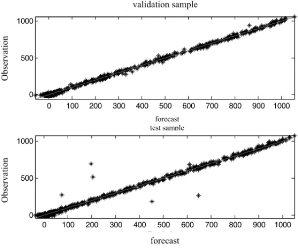
It is noteworthy that the wavelet decomposition of signals in the samples of training, validation and testing were done individually. In Figure 8, it is showed the scatter plots of the observations of global horizontal solar radiation and their forecasts by ANN (with input wavelet), for the validation and test samples.
5.3 Modeling for the 10 time series
Figure 5– (a) Global horizontal solar radiation at Cuiab´a.
neurons in the hidden layer for each time series. For both models (ANN and WD-ANN), it was calculated the Root Mean Square Deviation (RMSE) and the coefficient of determination R2for the training, validation and test periods. Almost all statistics for both periods show lower values of RMSE and higher values of R2for WD-ANN models when compared to the ANN models and na¨ıve predictor.
6 CONCLUSIONS
Figure 5– (b) Global horizontal solar radiation at Cuiab´a.
It could be seen that the forecasts derived from the WD-ANN method had a significantly higher correlation with the time series observations of global horizontal solar radiation when compared with the forecasts arising from the traditional ANN (i.e., without considering the wavelet signals as input patterns). It also showed the lower values of RMSE for almost all periods of interest.
0 100 200 300 400 500 600 700 800 900 0 200 400 600 800 1000
Amostra de Validação
Previsões O b s er v aç ões
0 100 200 300 400 500 600 700 800 900 0 200 400 600 800 1000
Amostra de Teste
Previsões O b s e rv aç ões validation sample forecast test sample forecast Observation Observation
Figure 6– Scatter plot between observed and forecasted values by ANN method.
0 1000 2000 3000 4000 5000 6000 7000 8000 9000
-1.5 -1 -0.5 0 0.5 1 pç approximation signals time
(a) Approximation component of levelm0−fVm0()(t)
8760
t=1
0 1000 2000 3000 4000 5000 6000 7000 8000 9000 -0.5 0 0.5 1 details signals time
(b) Details component of levelm0−fWm0(ω)(t)
8760
t=1
0 1000 2000 3000 4000 5000 6000 7000 8000 9000 -1 -0.5 0 0.5 details signals time
(c) Details component of levelm0+1fWm0+1(ω)(t)
8760
t=1
Table 2– Types of ANN, RMSE and R2for each time series’ modeling.
Local With Window
Neurons RMSE Wm−2 R2
wavelet? length in the Training Validation Test Training Validation Test hide layer
Bras´ılia
without 12 8 77,90 102,40 107,88 0,9352 0,8772 0,8707
db32 15 8 6,03 15,76 91,29 0,9996 0,9971 0,9074
Naive predictor 129,00 134,64 143,34 0,8302 0,7992 0,7848
Caic ´o
without 15 19 65,13 57,82 66,58 0,9616 0,9756 0,9648
db20 15 8 28,91 54,45 37,61 0,9924 0,9784 0,9888
Naive predictor 130,31 135,72 134,68 0,8523 0,8704 0,8611
Campo without 15 10 70,59 90,36 120,07 0,9416 0,9225 0,865
Grande db20 12 8 4,43 9,25 76,06 0,9998 0,9992 0,9458
Naive predictor 121,14 132,95 154,21 0,8354 0,8394 0,7898
Cuiab´a
without 10 19 62.8789 88.1219 106.2804 0.951 0.9199 0.8908
db38 10 12 8.354 20.4286 26.1382 0.9991 0.9957 0.9934
Naive predictor 113,55 129,76 144,84 0,8465 0,8340 0,8076
Florian´o- without 10 10 73.4169 96.9041 109.7201 0.9134 0.9114 0.8958
polis db40 8 15 4.8984 7.1704 50.12 0.9996 0.9995 0.9783
Naive predictor 107,10 130,99 143,29 0,8240 0,8447 0,8302
Joinville
without 11 5 64.2913 88.226 92.2426 0.892 0.8883 0.8625
db32 12 10 2.8592 6.4026 84.3426 0.9998 0.9994 0.885
Naive predictor 87,77 111,23 111,58 0,8087 0,8304 0,8089
Natal
without 15 5 76.9716 58.2249 57.3206 0.9434 0.9751 0.9759
db20 15 13 4.3326 5.2023 75.9577 0.9998 0.9998 0.9577
Naive predictor 129,73 133,72 133,36 0,8459 0,8728 0,8738
Palmas
without 15 10 71.2284 105.5357 101.7703 0.946 0.8849 0.8727
db40 10 13 5.5671 11.1399 60.3 0.9997 0.9987 0.9553
Naive predictor 126,70 149,35 138,54 0,8362 0,7829 0,7780
Petrolina
without 15 9 64.1714 69.3586 75.1056 0.9526 0.9605 0.9423
db15 9 20 3.6199 7.7754 82.5086 0.9998 0.9995 0.9303
Naive predictor 115,59 130,42 121,63 0,8520 0,8651 0,8543
S˜ao without 15 20 56.2227 71.8829 98.875 0.9562 0.9601 0.9329
Martinho db13 20 14 5.5941 10.4779 19.6784 0.9996 0.9992 0.9973
Naive predictor 100,11 126,80 140,37 0,8662 0,8798 0,8694
0 100 200 300 400 500 600 700 800 900 1000 0
500 1000
Amostra de Validação
Previsões
Ob
s
e
rv
a
ç
õ
e
s
0 100 200 300 400 500 600 700 800 900 1000
0 500 1000
Amostra de Teste
Previsões
O
bs
e
rv
aç
ões
validation sample
forecast test sample
forecast
Observation
Observation
Figure 8– Scatter plot between observed and forecasted values by WD-ANN method.
REFERENCES
[1] CAOS, WENGW, CHENJ, LIUW, YUG & CAOJ. 2009. Forecast of Solar Irradiance Using Chaos Optimization Neural Networks. Power and Energy Engineering Conference, Asia-Pacific, 21-31, Mar.
[2] CATALAO˜ JPS, POUSINHOHMI & MENDESVMF. 2011. Short-Term Wind Power Forecasting in Portugal by Neural Networks and Wavelet Transform.Renewable Energy,36: 1245–1251.
[3] CHAABENEM & AMMARBM. 2008. Neuro-Fuzzy Dynamic Model with Kalman Filter to Forecast Irradiance and Temperature for Solar Energy Systems.Renewable Energy,33(7): 1435–1443. [4] DAUBECHIESI. 1988. Orthonormal Bases of Compactly Supported Wavelet.Communications Pure
and Applied Math,41(7): 909–996.
[5] DENG F, SUG, LIU C & WANG Z. 2010. Global Solar Radiation Modeling Using The Artifi-cal Neural Network Technique.Power and Energy Engineering Conference, Chengdu, Asia-Pacific, 28-31, Mar.
[6] FARIADL, CASTROR, PHILIPPARTC & GUSMAO˜ A. 2009. Wavelet Pre-Filtering in Wind Speed Prediction.Power Engineering, Energy and Electrical Drives, POWERENG, International Confer-ence, Lisboa, Portugal, 19-20, Mar.
[7] HAYKINSS. 2001. Redes Neurais Princ´ıpios e Aplicac¸ ˜oes, 2a. edic¸˜ao. Porto Alegre.
[8] KRISHNAB, SATYAJIRAOYR & NAYAKPC. 2011. Time Series Modeling of River Flow Using Wavelet Neural Networks.Journal of Water Resource and Protection,3: 50–59.
[10] KUBRUSLY CS & LEVANN. 2002. Dual-Shift Decomposition of Hilbert Space. Semigroups of Operators: Theory and Application 2, 145–157.
[11] LEIC & RANL. 2008. Short-Term Wind Speed Forecasting Model for Wind Farm Based on Wavelet Decomposition. DRPT2008, Nanjing, China, 6-9, Apr.
[12] LEVANN & KUBRUSLYCS. 2003. A Wavelet “Time-Shift-Detail” Decomposition.Mathematics and Computers in Simulation,63(2): 73–78.
[13] LIUH, TIANHQ, CHENC & LIY. 2010. A Hybrid Statistical Method to Predict Wind Speed and Wind Power.Renewable Energy,35: 1857–1861.
[14] MALLATS. 1998. A Wavelet Tour of Signal Processing. Academic Press, San Diego.
[15] MINUKK, LINEESHMC & JESSYJOHNC. 2010. Wavelet Neural Networks for Nonlinear Time Series Analysis.Applied Mathematical Sciences,4(50): 2485–2495.
[16] OGDEN RT. 1997. Essential Wavelet for Statistical Applications and Data Analysis. Birkh¨auser, Boston.
[17] PERDOMOR, BANGUEROE & GORDILLOG. 2010. Statistical Modeling for Global Solar Radiation Forecasting in Bogot´a.Photovoltaic Specialists Conference (PVSC), Honolulu, HI, 20-25, Jun. [18] PEREIRAEB, MARTINSFR, ABREU, SL & RUTHERR. 2006. Atlas Brasileiro de Energia Solar.
S˜ao Jos´e dos Campos: INPE.
[19] REISAR & SILVAAPA. 2004. Aplicac¸˜ao da Transformada Wavelet Discreta na Previs˜ao de Carga de Curto Prazo via Redes Neurais.Revista Controle & Automac¸ ˜ao,15(1): 101–108.
[20] TEIXEIRA JUNIORLA, PESSANHAJFM & SOUZARC. 2011. An´alise Wavelet e Redes Neurais Artificiais na Previs˜ao da Velocidade de Vento. In:XLIII Simp´osio Brasileiro de Pesquisa Opera-cional, Ubatuba, S˜ao Paulo, 15-18, Aug.
[21] TEIXEIRA JUNIORLA, PESSANHAJFM, MENEZES ML, CASSIANOKM & SOUZARC. 2012. Redes Neurais Artificiais e Decomposic¸˜ao Wavelet na Previs˜ao da Radiac¸˜ao Solar Direta. In:
Simp´osio Brasileiro de Pesquisa Operacional, Rio de Janeiro, 24-28, Sep.
[22] WITTMANNM, BREITKREUZH, SCHROEDTER-HOMSCHEIDTS & ECKM. 2008. Case Studies on the Use of Solar Irradiance Forecast for Optimized Operation Strategies of Solar Thermal Power Plants.IEEE Journal of Selected Topics in Applied Earth Observations and Remote Sensing,1(1): 18–27.
[23] YANLINGG, CHANGZHENGC & BOZ. 2012. Blind Source Separation for Forecast of Solar Irra-diance.International Conference on Intelligent System Design and Engineering Application, Sanya, Hainan, 6-7, Jan.
[24] YONAA & SENJYU T. 2009. One-Day-Ahead 24-Hours Thermal Energy Collection Forecasting Based on Time Series Analysis Technique for Solar Heat Energy Utilization System. Transmission & Distribution Conference & Exposition: Asia and Pacific, Seoul, 26-30, Oct.
[25] ZERVASPL, SARIMVEISH, PALYVOSJA & MARKATOSNCG. 2008. Prediction of Daily Global Solar Irradiance on Horizontal Surfaces Based on Neural-Network Techniques.Renewable Energy,
33(8): 1796–1803.
[27] ZHOUH, SUNW, LIUD, ZHAOJ & YANGN. 2011. The Research of Daily Total Solar-Radiation