Economia Aplicada, v. 13, n. 4, 2009, pp. 463-479
THE STATIONARITY OF CONSUMPTION-INCOME
RATIOS: EVIDENCE FROM SOUTH AMERICAN
COUNTRIES
Fábio Augusto Reis Gomes*
Douglas de Souza Franchini†
Resumo
Este artigo analisa a ordem de integração da razão consumo-renda em 10 países da América do Sul. Para tanto, utilizamos o teste ADF e sua versão painel, além de um teste LM de raiz unitária com quebra estrutu-ral(s). Enquanto os primeiros testes encontraram evidências mais favorá-veis a processos integrados, após o controle de quebras estruturais apenas o processo do Uruguai parece ser integrado. Assim, em geral, a razão consumo-renda foi diagnosticada como um processo estacionário, como sugerido pelo modelo de hábito e pelas hipóteses de renda relativa, renda permanente e ciclo de vida.
Resumo
This paper analyzes the order of integration of the consumption-in-come ratio in 10 South American countries. To do this, the individual ADF test, its panel versions and the Minimum LM unit root test with structural break(s) were employed. While the former tests found more favorable evidence of an integrated process, after controlling for structural breaks only Uruguay seems to be integrated. Thus, in general, the consumption-income ratio was diagnosed as a stationary process, as suggested by the relative income hypothesis, the habit persistence model, the permanent income hypothesis and the life cycle hypothesis.
Keywords: Consumption-income ratio, unit root tests, structural break,
South America
JEL classification:C12, C22, E21.
*Insper Instituto de Ensino e Pesquisa. Address: Rua Quatá, 300, Sala 422, Vila Olímpia. São
Paulo, SP, Brazil. CEP: 04546-042. Email: [email protected]
†Insper Instituto de Ensino e Pesquisa
1
Introduction
The time series properties of the consumption-income ratio or the average propensity to consume – hereafter APC - are a controversial issue on the-oretical grounds. The Keynesian absolute income hypothesis, the Marxian underconsumption theory, and Deaton’s (1977) involuntary savings theory imply an integrated APC. The relative income hypothesis, the habit persis-tence model, the permanent income hypothesis and the life cycle hypothesis lead to a stationary APC. An integrated behavior means that policy shocks are likely to have a permanent effect on the APC. On the other hand, the
station-ary case implies the existence of a long-run equilibrium relationship between consumption and income, which means both that APC has a mean reversion behavior and shocks have temporary effects.
On empirical grounds, these conflicting predictions that have been evalu-ated by means of unit root tests and the results are also controversial.Molana
(1991),Drobny & Hall(1989) andHall & Patterson (1992) analyzed the UK
case using the Augmented Dickey–Fuller (ADF) unit root test and their find-ings indicate that APC is non-stationary. Horioka(1997) reached the same result for Japan, applying the ADF test. Applying the same test, King et al.
(1991) reached the opposite conclusion for the US economy. In addition,
Ungern-Stemberg’s (1986) findings indicated that UK and Germany present a
stationary APC.
A feature of these earlier papers is the use of the ADF test to investigate the order of integration of APC. Currently, the ADF problem of low-power is well-known. To overcome it, the following literature has used more powerful tests, like panel and asymmetric unit root tests. Sarantis & Stewart(1999) analyzed 20 OECD countries using panel unit root tests and still obtained non-stationary proceses for all these. Cook(2003) confirmed this result for the UK – a country studied by Sarantis & Stewart (1999)–, using powerful modifications of the ADF test: the weighted symmetric Dickey–Fuller test
(Park & Fuller (1995)) and the recursive mean adjusted Dickey–Fuller test
(Shin & So(2001)).
Applying recent advances in panel and asymmetric unit root tests,Tsionas
& Christopoulos(2002), studied 14 European countries analyzed bySarantis
& Stewart(1999). Initially, the panel unit roots tests supported the
hypothe-sis of a unit root in the APC. However, taking into account the presence of an asymmetric adjustment, it was found that stationarity prevails in at least one regime for each country. Thus, the asymmetric unit root test offers less
evi-dence in favor of the unit root hypothesis. However,Cerrato & Stewart(2008) analyzed 24 OECD and 33 non-OECD countries using nonlinear panel unit root tests and the results suggested that, for both groups, the majority of the series areI(1).
Cook (2005) examined the same sample that Sarantis & Stewart(1999) addressed, applying unit root tests with structural changes and reversed pre-vious findings of non-stationarity, rejecting the unit root hypothesis for all 20 OECD economies. Both works share the same concern about the ADF test: the lack of power could be the reason behind the non-rejection of the unit root null hypothesis. However, whileSarantis & Stewart(1999) attempted to solve the problem using powerful panel tests,Cook(2005) considered the omission of structural breaks as the source of the lower power. Indeed, Perron(1989,
Stationarity of Consumption-Income Ratio 465
of integration of economic series in the presence of structural changes. Fi-nally, whileSarantis & Stewart(1999) did not reject the unit root hypothesis,
Cook(2005) did.
As the literature has focused on developed countries, there is a lack of in-formation about underdeveloped ones.1To fulfill this need, this paper inves-tigates the APC properties of 10 South American economies, using the ADF test as a benchmark and its panel versions fromMaddala & Wu(1991) and
Choi(2001). Furthermore, the possibility of structural breaks is taken into account by means of the Minimum LM unit root test with one and two struc-tural break(s) as inLee & Strazicich(1999) andLee & Strazicich(2003), re-spectively.
To preview the main findings of the paper, while the individual ADF test and its panel versions found evidence suggesting an integrated APC, after controlling for structural breaks the evidence indicate just the opposite. In-deed, modeling a broken trend, only Uruguay seems to be integrated. Then, apart from this country, shocks to the APC seem to be temporary, as suggested by the permanent income and the life cycle hypotheses. These hypotheses are especially important because they embedded an idea presented in virtually all economics model: consumers desire to smooth their consumption path.
The paper is organized as following. The second section presents the econometric methodology and the data set. The third section displays the results. Lastly, the conclusions are summarized.
2
Econometric Methodology
2.1 Unit Root Tests
To examine the APC order of integration, the ADF test is used as a benchmark
(Dickey & Fuller 1979). The test equation for each country takes the following
form,
∆yt=µ+βt+αyt −1+
k
X
j=1
cj∆yt−j+εt
whereyt is the logarithm of the consumption income ratio. The lags of the dependent variable used to correct serial correlation, the Schwarz information criterion is employed on setk. The maximum value allowed forkis 8.2
In an attempt to increase the power of the ADF test, its panel versions ac-cording toMaddala & Wu(1991) andChoi(2001) were employed. Maddala
& Wu(1991) used theFisher’s (1932) results to derive a test that combine the
p-values from individual ADF tests. Defineπi as thep-value from any in-dividual unit root test for cross-section i, i = 1, ..., N. Then, under the null hypothesis of unit root for allNcross-sections, the following asymptotic re-sult is valid
−2 N
X
i=1
log (πi)→χ22N (1)
1The exception is Cerrato et al (2008) which, unlike our work, does not take into account
structural breaks.
In addition,Choi(2001) demonstrated that:
1
√
N
N
X
i=1
Φ−1(π
i)→N(0,1)
whereΦ−1is the inverse of the standard normal cumulative distribution
func-tion. Thus, based on individual ADF p-values, both panel tests can be con-ducted. It’s worth noting that the null hypothesis of both tests is the presence of unit root for each country while the alternative hypothesis is stationary for some (not necessarily all) of them. Thus, if the null hypothesis is not rejected, it means that it is not possible to reject that all countries present an integrated APC. However, rejection of the null hypothesis does not imply that all coun-tries are characterized by a stationary APC.3
FromPerron(1989), it is well known that the ADF unit root test can fail
to reject a false unit root due to misspecification of the deterministic trend function. Indeed, Perron(1989,1997), Zivot & Andrews(1992) and
Lums-daine & Papell(1997) extended the ADF test allowing exogenous/endogenous
break(s), in an attempt to circumvent this drawback. However, these efforts
were not absolutely successful, once the critical values of their unit root tests were derived assuming no break(s) under the null hypothesis, which leads to a spurious rejection of the null hypothesis when there is a unit root with breaks (Lee & Strazicich 2001,2003).
Lee & Strazicich(1999,2003) developed a one-break and two-break
mini-mum LM unit root test, respectively, the properties of wich are unaffected by
break(s) under the null hypothesis, avoiding both the spurious rejection and the trend misspecification. Hence, to investigate the order of integration of the APC series the tests fromLee & Strazicich(1999,2003) are employed. Ac-cording to the LM (score) principle, a unit root test statistic can be obtained from the regression:4
∆yt=d′∆Zt+φS˜t −1+
k
X
i=1
γi∆S˜t−i+εt
where ˜St is a de-trended series such that ˜St =yt−ψ˜x−Ztδ˜, t = 2, ..., T and
∆S˜
t−i,i= 1, ..., k, terms are included to correct serial correlation. For setk, the general-to-specific approach is used. According toNg & Perron(1995),k is chosen using the 10% value of the asymptotic normal distribution, 1.645, to evaluate the significance of the last lag. The upper bound forkis 8. Consid-ering 2 changes in level and trend (Model C), the components of ˜St are: (i)
Zt = [1, t, D1t, D2t, DT1∗t, DT2∗t]′ withDjt = 1 fort≥TBj+ 1,j = 1,2, and zero otherwise; DT∗
jt =tfort≥TBj+ 1,j= 1,2, and zero otherwise; TBjstands for the time period of the breaks; (ii) ˜ψx =y1−Z1δ˜, where y1 and Z1 are the
first observations of yt andZt, respectively; (iii) ˜δis a vector of coefficients in the regression of∆y
t on∆Zt= [1, B1t, B2t, D1t, D2t]′, whereBjt =∆Djt and
Djt =∆DTjt∗,j= 1,2.
3It is worth mentioning that both tests -Maddala & Wu(1991) andChoi(2001) - are based
on the assumption that the error terms are not cross-correlated.
4Due to space limitation only the two-break test is explained. For the one break
Stationarity of Consumption-Income Ratio 467
The unit root null hypothesis is described in equation (1) byφ= 0 and the test statistic is defined by ˜τ, the t-statistic for the null hypothesisφ = 0. To endogenously determine the location of the break points,TBj, a grid search is used to minimize t-test statistic. There is a repeated procedure at each combi-nation of the break points (λj=TBj/T,j= 1,2) over the time interval [.1T , .9T] whereT is the sample size. Lastly, the critical values depend on the location of the breaks and are provided forT = 100 byLee & Strazicich(1999) andLee
& Strazicich(2003) for one-break and two-break tests, respectively.
FollowingStrazicich et al.(2001) , the relevance of each break date is eval-uated using the t-test statistic. If the level (Bjt) and the trend (Djt) dummies are not relevant for one of the break dates, the one-break test is used. If the remaining break is not relevant, the ADF test constitutes an appropriate test, once no structural break was detected.
It is worth noting that, a structural change in APC is compatible with the permanent income and life cycle hypotheses, for instance. An abrupt change in APC occurs when there is a change in income (consumption) that is not followed by a similar change in consumption (income). Indeed, these theories imply that changes in income cause changes in consumption only if perma-nent income is altered. Thus, if income changes, but permaperma-nent income does not vary, then consumption remains constant and, as a result, a structural break in the APC might occur. Also, permanent income can change while the current income is stable and, as a consequence, the APC changes. Therefore, as interpreted by Cook(2005), a stationary APC around a broken trend can be viewed as evidence in favor of the consumption theories mentioned.
2.2 The Data Set
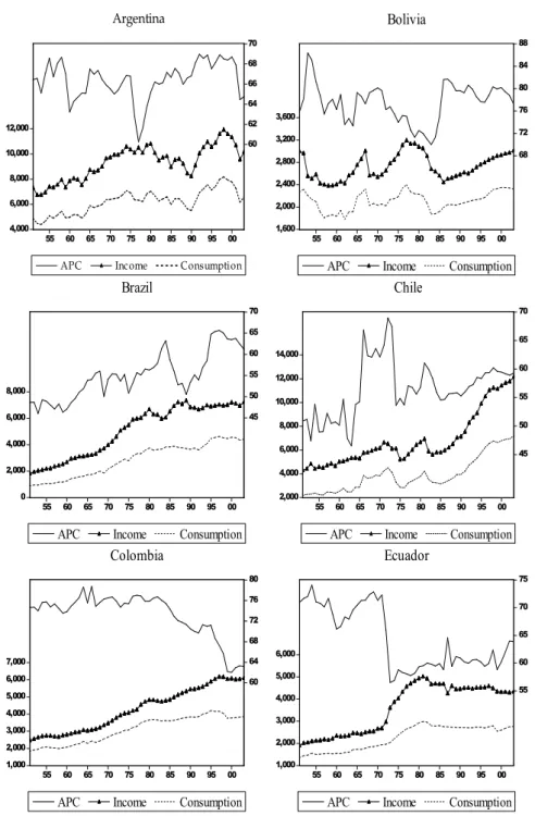
The data set was extracted from Penn World Table 6.2 and refers to the an-nual income (RGDPL) and the anan-nual ratio of consumption and income (KC), both ranging from 1951 to 2003. The KC refers to the consumption share of RGDPL. Ten South American countries were examined: Argentina, Bolivia, Brazil, Chile, Colombia, Ecuador, Paraguay, Peru, Uruguay and Venezuela. The others South American countries were ignored due to the lack of data over some periods.
in-Figure 1: APC, Consumption and Income Evolution 4,000 6,000 8,000 10,000 12,000 60 62 64 66 68 70
55 60 65 70 75 80 85 90 95 00
APC Income Consumption
Argentina 1,600 2,000 2,400 2,800 3,200 3,600 68 72 76 80 84 88
55 60 65 70 75 80 85 90 95 00
APC Income Consumption
Bolivia 0 2,000 4,000 6,000 8,000 45 50 55 60 65 70
55 60 65 70 75 80 85 90 95 00
APC Income Consumption
Brazil 2,000 4,000 6,000 8,000 10,000 12,000 14,000 45 50 55 60 65 70
55 60 65 70 75 80 85 90 95 00
APC Income Consumption
Chile
1,000 2,000 3,000 4,000 5,000 6,000 7,000 60 64 68 72 76 80
55 60 65 70 75 80 85 90 95 00
APC Income Consumption
Colombia 1,000 2,000 3,000 4,000 5,000 6,000 55 60 65 70 75
55 60 65 70 75 80 85 90 95 00
APC Income Consumption
Ecuador
ternational creditors that had been financing their development in previous years. The debt crisis began when the international capital markets became aware that Latin American countries would not be able to pay back their loans, which occurred in 1982 when Mexico declared default.
Stationarity of Consumption-Income Ratio 469
Figure 1: Continued.
1,000 2,000 3,000 4,000 5,000 6,000
70 75 80 85 90 95
55 60 65 70 75 80 85 90 95 00
APC Income Consumption Paraguay
1,000 2,000 3,000 4,000 5,000 6,000
40 50 60 70 80
55 60 65 70 75 80 85 90 95 00
APC Income Consumption Peru
2,000 4,000 6,000 8,000 10,000 12,000
60 64 68 72 76 80
55 60 65 70 75 80 85 90 95 00
APC Income Consumption Uruguay
0 2,000 4,000 6,000 8,000 10,000
30 40
50 60 ✡0
55 60 65 ✡0 ✡5 80 85
☛0 ☛5 00
APC Income Consumption Venezuela
generate a common pattern among them. For instance, after a negative break around 1985 - which reached its lowest value in Sarney’s 1989 external debt moratorium , Brazil’s APC seemed to recover it previous pattern in approx-imately 1994, when the successful Real Stabilization Plan was implemented. Another example is the death of Bolivian President René Barrientos Ortuño in 1969 and the subsequent military coup d’etat in 1971, which suspended its political activities. It can be noted that Bolivia’s APC started to decrease around these years.
Ben-David & Loewy(1998) andFerreira et al.(2009) analyzed the presence
of structural breaks in income growth and total factor productivity, respec-tively. Both works included some Latin American countries and supported the relevance of external shocks - oil shocks and the debt crisis -, as possible sources of the breaks. Following these works, we have analyzed the temporal distribution of the breaks, keeping in mind relevant historical events. How-ever, this exercise can not be viewed as a causality test.
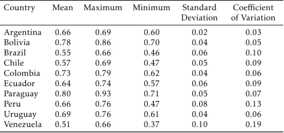
Country Mean Maximum Minimum Standard Deviation
Coefficient
of Variation
Argentina 0.66 0.69 0.60 0.02 0.03
Bolivia 0.78 0.86 0.70 0.04 0.05
Brazil 0.55 0.66 0.46 0.06 0.10
Chile 0.57 0.69 0.47 0.05 0.09
Colombia 0.73 0.79 0.62 0.04 0.06
Ecuador 0.64 0.74 0.57 0.06 0.09
Paraguay 0.80 0.93 0.71 0.05 0.07
Peru 0.66 0.76 0.47 0.08 0.13
Uruguay 0.69 0.76 0.61 0.04 0.06
Venezuela 0.51 0.66 0.37 0.10 0.19
Table 1: APC: Descriptive Statistics
in 1994. The minimum value is 0.460, corresponding to Brazil in 1953, one year before the president, Getulio Vargas, committed suicide. The countries with larger standard deviations and coefficients of variation are Peru and
Venezuela; indeed they seem to present structural breaks that leverage the dispersion measures. Peru presented an upward trend until mid-1960, when it flattened. Venezuela started a huge increase in the 70s, which stabilized in the early 80s.
3
Empirical Results
The results from the ADF test are reported in Table2. At the 5% level, the unit root null hypothesis is rejected only for Argentina and Paraguay. Increasing the significance level to 10%, Chile and Peru also diverfe from the unit root hypothesis.5 Thus, in general, there are evidences in favor of a non-stationary
APC.
The panel versions of ADF test are shown in Table2. Considering a con-stant and a linear trend for all countries, Fisher and Choi tests did not reject the unit root null hypothesis for all countries, at the 5% level. Considering only a constant as a deterministic term, the Choi test reached the same con-clusion. Thus, the panel tests tend to suggest that APC is an integrated pro-cess. The exception was the Fisher test when the linear trend is not included, that the unit root null hypothesis is rejected at the 5% level of significance. If, on the one hand, the panel tests have better power properties, on the other hand, they also are uninformative about which series are stationary when the null hypothesis is rejected. As discussed byBreuer et al.(2001) and Chang
et al.(2005), these panel tests are incapable of determining the mixing ofI(0)
andI(1) series in a panel setting, which constitutes their major disadvantage. The overall picture suggests that APC is an integrated process, at least, for most countries. However, it is imperative to control for possible structural changes, once its omission leads to a bias in favor of the unit root null hypoth-esis. This bias is, in general, mainly important for the economies analyzed,
5The significance of the ADF test statistics is established via comparison with the critical
S ta tio n ar ity of C on su m p tio n -I n co m e Ra tio 4 7 1
Table 2: ADF and Minimum LM Two Breaks Unit Root Tests
Individual Unit Root Tests
Country
ADF test Statistic
LM Two Breaks
LM Test Statistic
First Break Second Break
Year B1 D1 Year B2 D2
Argentina −3.377∗ −4.981 1979 −0.002
(−0.1) 0.004(0.7) 1995 0.014(0.73) −(−0.0040.55) Bolivia −2.587 −8.518∗ 1969 0.067∗
(3.17) −0.028 ∗
(−3.68) 1984 −(−0.0321.65) 0.119 ∗ (8.52) Brazil −2.901 −6.630∗∗ 1983 0.110∗
(3.14) −0.083 ∗
(−5.42) 1998 −(−0.0581.49) 0.086 ∗ (3.47) Chile −2.832∗ −7.058∗∗ 1964 −0.156∗
(−2.86) 0.201 ∗
(5.65) 1974 0.014(0.3) −0.157 ∗ (−5.41) Colombia −1.301 −6.530∗∗ 1978 −0.029∗
(−2.16) 0.010 ∗
(2.03) 1997 0.022(1.44) −0.033 ∗ (−3.9) Ecuador 0.062 −7.624∗∗ 1971 0.004
(0.14) −0.078 ∗
(−6.15) 1985 −(−0.0883.37) 0.122 ∗ (7.43) Paraguay −3.788∗∗ −7.237∗∗ 1965 −0.007
(−0.25) −0.027 ∗
(−2.05) 1978 −0.208 ∗
(−7) −2.047 ∗ (6.34) Peru −1.635∗ −8.318∗∗ 1966 −0.142∗
(−4.97) 0.103 ∗
(6.1) 1978 0.038(1.96) −0.056 ∗ (−5.59) Uruguay −0.065 −5.641∗ 1970 −0.027
(−1.1) 0.011(1) 1978 −0.054 ∗
(−2.53) 0.013(1.38) Venezuela −1.126 −6.443∗∗ 1968 0.118∗
(2.84) −0.122 ∗
(−4.1) 1981 0.024(0.65) 0.068 ∗ (3.38)
Determinist Terms
Determinist Terms ADF - Fischer ADF - Choi
Constant and Trend 26.58 −0.89 Constant 31.994∗ −1.569∗
Table 3: Minimum LM One Break Unit Root Test
Country LM Test Statistic
Break
Year B1 D1
Argentina −4.597∗∗ 1979 −0.009
(−0.455) 0.015
∗
(−2.561)
Uruguay −3.820 1977 −0.017
(−0.673) −(−01..018846) Note: The one break LM test corresponds to Model C (level and trend changes). The LM test chooses k following Ng and Perron (1995) with a critical value of 1.645 (standard normal distribution with 5% significance). The symbols∗and∗∗denote statistical significance at the 10% and 5% levels, respectively.
given the instability of the South America countries. The results from the two-break LM test are reported in Table2. First, notice that, based on t-statistic, all countries have at least one dummy relevant at 5%, in each break trend, except for Argentina and Uruguay. This result reflects the importance to control for structural changes for: Bolivia, Brazil, Chile, Colombia, Ecuador, Paraguay, Peru and Venezuela. These 8 countries present a stationary APC, at the 5% level. The significance of the stated LM test statistics is established via com-parison with the critical values fromLee & Strazicich(2003).
Argentina and Uruguay cases were re-estimated by means of the one-break LM test, as reported in Table3. For Argentina, only the dummy variableD1
is relevant at the 5% level, and the LM statistic rejected the unit root null hypothesis at the 5% level.6 Uruguay presents an additional difficulty: the
dummy variableD1is significant only at the 10% level. If the break is
consid-ered relevant, which seems to be the case based on Figure2, the LM statistic did not reject the unit root null hypothesis.7 If the break is considered irrele-vant, the ADF test can be used and, as noted, this test did not reject the unit root null hypothesis.
Therefore, once structural change is incorporated into the analysis, the APC is found to be stationary for all of the economies considered except Uruguay. Rejection of the unit root hypothesis is emphasized by the rela-tively short span of data, which might be expected to result in a reduction of the power of the test.
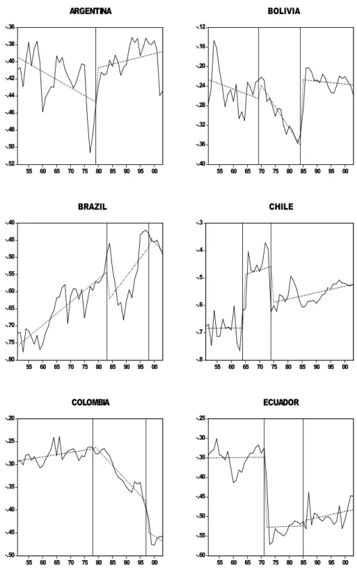
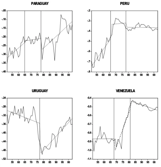
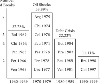
A look at the countries in Figure2provides a visual illustration of the es-timated broken trend. Figure2 displays the break points identified by the one/two-break tests reported in Table1and Table2and plots the logarithm of the APC series and its trend function. The broken trends were estimated via ordinary least squares to connect the break points.
To see the distribution of the break dates, Figure3presents a kind of his-togram of them. From 32 breaks, 5 occurred in the 1960s; 7 in the 1970s; 4 in the 1980s and 2 in the 1990s. As mentioned, some of them could be attributed to external issues, like the oil shocks, that caused a hike in energy prices. Note that Chile and Ecuador present a break at the beginning of the 70s, while Ar-gentina, Colombia, Paraguay, Peru and Uruguay presented a break in the end of the 70s. Another important external shock was the onset of the debt crisis
6The significance of the stated LM test statistics is established via comparison with the critical
values ofLee & Strazicich(1999).
Stationarity of Consumption-Income Ratio 473
-.52 -.50 -.48 -.46 -.44 -.42 -.40 -.38 -.36
55 60 65 70 75 80 85 90 95 00 ARGENTINA
-.40 -.36 -.32 -.28 -.24 -.20 -.16 -.12
55 60 65 70 75 80 85 90 95 00 BOLIVIA
-.80 -.75 -.70 -.65 -.60 -.55 -.50 -.45 -.40
55 60 65 70 75 80 85 90 95 00 BRAZIL
-.8 -.7 -.6 -.5 -.4 -.3
55 60 65 70 75 80 85 90 95 00 CHILE
-.50 -.45 -.40 -.35 -.30 -.25 -.20
55 60 65 70 75 80 85 90 95 00 COLOMBIA
-.60
-.55 -.50 -.45 -.40 -.35 -.30 -.25
55 60 65 70 75 80 85 90 95 00 ECUADOR
-.40 -.35 -.30 -.25 -.20 -.15 -.10 -.05
55 60 65 70 75 80 85 90 95 00
PARAGUAY
-.8 -.7 -.6 -.5 -.4 -.3 -.2
55 60 65 70 75 80 85 90 95 00
PERU
-.52 -.48
-.44 -.40 -.36 -.32 -.28
-.24
55 60 65 70 75 80 85 90 95 00
URUGUAY
-1.1 -1.0 -0.9 -0.8 -0.7 -0.6 -0.5 -0.4
55 60 65 70 75 80 85 90 95 00
VENEZUELA
Figure 2: (ln) APC Evolution, Trend Function and Break Dates (continued)
in 1982. Bolivia, Brazil, Ecuador and Venezuela presented a break close to this year. Thus, in this sense, approximately 60% of the breaks can potentially be attributed to external shocks.
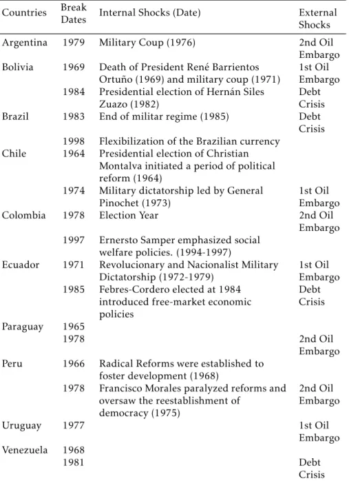
Internal shocks are also able to change the APC pattern. For each country we look for internal events close to the estimated break dates. These events along with the external shocks are listed in Table 4 for interested readers. The analysis of external and internal shocks does not constitute a causality test. However, this attempt to offer possible explanations for breaks that are
relevant should be noted because, when there are few observations in a series, the model can over-fit the data, finding breaks that may not exist.
4
Conclusions
mod-Stationarity of Consumption-Income Ratio 475
Table 4: Internal and External Shocks
Countries Break
Dates Internal Shocks (Date) ExternalShocks
Argentina 1979 Military Coup (1976) 2nd Oil Embargo Bolivia 1969 Death of President René Barrientos
Ortuño (1969) and military coup (1971)
1st Oil Embargo 1984 Presidential election of Hernán Siles
Zuazo (1982)
Debt Crisis Brazil 1983 End of militar regime (1985) Debt
Crisis 1998 Flexibilization of the Brazilian currency
Chile 1964 Presidential election of Christian Montalva initiated a period of political reform (1964)
1974 Military dictatorship led by General Pinochet (1973)
1st Oil Embargo
Colombia 1978 Election Year 2nd Oil
Embargo 1997 Ernersto Samper emphasized social
welfare policies. (1994-1997)
Ecuador 1971 Revolucionary and Nacionalist Military Dictatorship (1972-1979)
1st Oil Embargo 1985 Febres-Cordero elected at 1984
introduced free-market economic policies
Debt Crisis
Paraguay 1965
1978 2nd Oil
Embargo Peru 1966 Radical Reforms were established to
foster development (1968)
1978 Francisco Morales paralyzed reforms and oversaw the reestablishment of
democracy (1975)
2nd Oil Embargo
Uruguay 1977 1st Oil
Embargo Venezuela 1968
1981 Debt
Number of Breaks
2 4 5 7
1960-1969 1970-1979 1980-1989 1990-1999 Ven 1969
Per 1966 Par 1965 Chi 1964 Bol 1969
Uru 1977 Per 1978 Par 1978 Ecu 1971 Col 1978 Chi 1974 Arg 1979
Ven 1981 Ecu 1985 Bra 1983 Bol 1984
Col 1997 Bra 1998 27.78%
Oil Shocks 38.89%
Debt Crisis 22.22%
11.11%
Figure 3: Histogram of Break Dates
eling of consumption functions, our understanding of savings behavior and business cycles, and economic policy. The presence (lack) of mean reversion implies that policy shocks are likely to have transitory (permanent) effects on
the APC in South American countries.
First of all, the individual ADF test and the panel versions were employed, finding evidence more favorable to the unit root case. However, the minimum LM unit root break test reverses these results in favor of stationary APC, ex-cept in case of Uruguay. Thus, after changes in trend function were prop-erly controlled for, the evidence of mean reversion in nine countries emerged, which is in line with the permanent income and the life cycle hypotheses. In summary, the evidence indicated out that policy shocks are likely to have temporary effects on the South American countries’ APC, except in Uruguay.
Bibliography
Ben-David, D. & Loewy, M. (1998), ‘Free trade growth and convergence.’,
Journal of Economic Growth3, 143–170.
Breuer, B., McNown, R. & Wallace, S. (2001), ‘Misleading inferences from panel unit-root tests with an illustration from purchasing power parity.’, Re-view of International Economics9, 482–493.
Cerrato, M. & Stewart, C. P. C. (2008), Is the consumption-income ratio sta-tionary? evidence from a nonlinear panel unit root test for oecd and non-oecd countries., Technical report, University of Glasgow.
Stationarity of Consumption-Income Ratio 477
Choi, I. (2001), ‘Unit root tests for panel data.’,Journal of International Money and Finance20, 249–272.
Cook, S. (2003), ‘The nonstationarity of the consumption-income ratio: Ev-idence from more powerful dickey–fuller tests.’, Applied Economics Letters 10, 393–395.
Cook, S. (2005), ‘The stationarity of consumption–income ratios: Evidence from minimum lm unit root testing.’,Applied Economics Letters89, 55–60.
Deaton, A. S. (1977), ‘Involuntary saving through unanticipated inflation’,
American Economic Review6, 899–910.
Dickey, D. & Fuller, W. (1979), ‘Distribution of the estimators for autoregres-sive time series with a unit root.’,Journal of the American Statistical Association 74, 427–731.
Drobny, A. & Hall, S. (1989), ‘An investigation of the long-run properties of aggregate nondurable consumers’ expenditure in the united kingdom.’,
Economic Journal99, 454–460.
Ferreira, P., Junior, A. G. & Pessôa, S. (2009), The effects of external and
internal shocks on total factor productivity. MIMEO.
Fisher, R. (1932),Statistical Methods for Research Workers, Edinburgh: Oliver & Boyd.
Hall, S. & Patterson, K. (1992), ‘A systems approach to the relationship be-tween consumption and wealth.’,Applied Economics24, 1165–1171.
Horioka, C. (1997), ‘A cointegration analysis of the impact of the age struc-ture of the population on the household saving rate in japan’,Review of Eco-nomic and Statistics79, 511–515.
King, R., Plosser, C., Stock, J. & Watson, M. (1991), ‘Stochastic trends and economic fluctuations.’,American Economic Review81, 819–840.
Lee, J. & Strazicich, M. (1999), Minimum lm unit root test. faculty research paper 9932, department of economics„ Technical report, University of Cen-tral Florida.
Lee, J. & Strazicich, M. (2001), ‘Break point estimation and spurious rejec-tions with endogenous unit root tests.’,Oxford Bulletin of Economic and Statis-tics63, 513–615.
Lee, J. & Strazicich, M. (2003), ‘Minimum lm unit root test with two struc-tural breaks.’,Review of Economic and Statistics85, 1082–1089.
Lumsdaine, R. & Papell, D. (1997), ‘Multiple trend breaks and the unit-root hypothesis.’,Review of Economics and Statistics79, 212–218.
MacKinnon, J. (1996), ‘Numerical distribution functions for unit root and cointegration tests.’,Journal of Applied Econometrics11, 601–618.
Molana, H. (1991), ‘The time series consumption function: error correction, random walkand the steady state.’,Economic Journal101, 382–403.
Ng, S. & Perron, P. (1995), ‘Unit root tests in arma models with data-dependent methods for the selection of the truncation lag.’, Journal of the American Statistical Association90, 269–281.
Park, H. & Fuller, W. (1995), ‘Alternative estimators and unit root tests for the autoregressive process.’,Journal of Time Series Analysis16, 415–429.
Perron, P. (1989), ‘The great crash, the oil price shock, and the unit root hypothesis.’,Econometrica57, 1361–1401.
Perron, P. (1997), ‘Further evidence on breaking trend functions in macroe-conomic variables.’,Journal of Econometrics80, 355–385.
Sarantis, N. & Stewart, C. (1999), ‘Is the consumption–income ratio station-ary? evidence from panel unit root tests.’,Economics Letters64, 309–314.
Shin, D. & So, B. (2001), ‘Recursive mean adjustment for unit root tests.’,
Journal of Time Series Analysis22, 595–612.
Strazicich, M., Lee, J. & Day, E. (2001), ‘Are incomes converging among oecd countries? time series evidence with two structural breaks.’, Journal of Macroeconomics26, 131–145.
Tsionas, E. & Christopoulos, D. (2002), ‘Non?sationarity in the consump-tion?income ratio: Further evidence from panel and assymetric unit root tests’,Economics Bulletin3, 1–5.
Ungern-Stemberg, T. (1986), ‘Inflation and the consumption function’, Re-view of World Economics (Weltwirtschaftliches Archiv)122, 741–744.