Equity Research : Cimpor

(1)

MASTERS OF SCIENCE IN BUSINESS ADMINISTRATION

EQUITY RESEARCH: CIMPOR

TOMÁS LAVIN PEIXE 152110052

ADVISOR: PROF. JOSÉ TUDELA MARTINS

Dissertation submitted in partial fulfillment of requirements for the degree of International MSC in Business Administration, at Universidade Católica Portuguesa, September, 2012

(2)

I. Preface

The goal of this dissertation is to value Cimentos de Portugal, SGPS, S.A, hereon stated as Cimpor. In order to do that, the main valuation methods and theories will be reviewed and consequently applied to deliver an investment recommendation regarding FY2012 stock price.

The structure of this dissertation is divided into eight main sections:

I. In the first section -executive summary- an equity research report will be presented summarizing Cimpor’s valuation as well as my final recommendation;

II. In section two -literature review- I will start by explaining the main role of valuation and then discuss the five major steps to value a firm (understanding the business, forecasting company performance, selecting the valuation model, converting forecast into valuation and making the investment decision);

III. In the third section, a detailed analysis of Cimpor will be presented covering the following topics: history, geographic diversification, growth strategy, shareholder structure, share performance and dividend policy;

IV. In the fourth section, an overview of cement industry will be done including an analysis of both past trends and future perspectives. Moreover, the main players and the Porter’s five forces analysis will be introduced;

V. Section five will show the main macroeconomic indicators needed to perform the valuation;

VI. In section six, Cimpor’s valuation will be computed through a DCF WACC based approach. In addition, a sensitivity analysis will be done as well as a relative valuation using EV/EBITDA and P/E multiples;

VII. In section seven, my own assumptions and results will be compared with an equity research report from BPI;

VIII. Finally, in the last section the main conclusions achieved will be summarized.

(3)

II. Acknowledgements

During the development of this dissertation, I had the pleasure to contact with a number of people that were crucial by the support and learning experience provided, to who I would like to acknowledge:

First of all, I would like to express my gratitude to Professor Aswath Damodaran for his constant availability to answer my questions, for providing all his MBA valuation classes online as well as all financial data used in this thesis.

I also want to recognize the availability and helpful feedback provided by Professor José Tudela Martins, BPI Equity Research team and Cimpor Investor Relations Department, for the additional data provided.

Finally, I would also like to thank to my family and Margarida Ramos for supporting me throughout my University studies.

(4)

6.3.8. Mozambique ...48 6.3.9. South Africa ...48 6.3.10. China ...48 6.3.11. India ...49 6.3.12. Cape Verde ...49 6.4. Sum-of-the-Parts ...49 6.5. Sensibility Analysis ...50 6.6. Relative Valuation ...51 6.7. Final Recommendation ...53 7. Valuation Comparison ... 54 8. Conclusion ... 56 9. Appendixes ... 57 10. References ... 76

(6)

1. Executive Summary

Equity Research

Msc in BA- Major in Finance

Cimpor

Building Materials

Student: Tomás Peixe

Company Report

September 5TH 2012

Protected by emerging markets

Emerging markets growth…

…Offset Iberia contraction

• We initiate our coverage on Cimpor with a target price of 5,16€, which represents a 6% downside potential comparing with the current price of 5,50€

• Cimpor’s solid operational results are a consequence of its geographical diversification (12 countries) and high exposure to emerging markets (78% of firm’s EBITDA)

• Cement consumption growth in emerging markets tends to be better than developed markets

• EBITDA margins continue at the top of the industry 26%

• Investment grade sustained and risk decoupled from sovereign.

Company description

Cimentos de Portugal - Cimpor is a Portuguese company that is ranked among the world top ten cement producers. In 2011 Cimpor employed 8255 employees with revenues of 2275€ million and a production capacity of 36,6 million tons.

(7)

2. Literature Review 2.1. The Role of Valuation

Understanding the tools to value a company as well as identifying its value drivers are mandatory fundamentals for anyone involved in the corporate finance field (Fernandez 2007). Damodaran (1994) also shares this view by saying, “knowing the value of an asset and what determines that value is a prerequisite for intelligent decision making”.

Despite the fact that valuation methods can be applied for a wide range of purposes such as mergers and acquisitions, identification of value drivers or to make strategic decisions (Fernandez 2007), this dissertation will be only focused on equity valuation.

The main scope of equity valuation is to help investors selecting stocks, especially fundamental analysts who believe that “the true value of the firm can be related to its financial characteristics: its growth prospects, risk profile and cash flows” (Damodaran 1994). Fernandez (2007) explains fundamental analysis as the valuation practice that “compares the value obtained with the share’s price on the stock market and to decide whether to buy, sell or hold the shares”.

In the recent decades, with the automation of stock exchanges and increasing popularity of stocks, more people has been discussing which is the best way to make investment decisions. This discussion started in 1934 when Benjamin Graham and David Dodd wrote Security Analysis for “all those who have a serious interest in security values”. In their book they considered that even taking into account the subjectivity of valuations and the difficulties to forecast companies performances, it is better to “invest based on a valuation method than in superficial analysis, market popularity, or business anticipations of short term”. They also highlighted that valuation methods are not supposed to present quick gains but should be used within a long-term perspective.

2.2. The Valuation Process

Penman (2001) defines fundamental analysis as the method that values a company through analyzing information and consequently extrapolating forecasts from that information. This

(8)

process, according to Stowe, Robinson, Pinto and McLeavey (2002) can be divided in the following 5 steps:

I. Understanding the business; II. Forecasting company performance; III. Selecting the valuation model; IV. Converting forecast to valuation;

V. Making the investment decision.

In this dissertation points 3 and 4 will be analyzed together since the process to convert forecast into valuation depends on the valuation model chosen.

2.2.1. Understanding the Business

Understanding the business model of the company as well as the industry in which the firm operates is one of the primary tasks for any analyst (Penman 2001). Before starting forecasting the company performance or choosing the valuation model, it is necessary to study not only the past financial statements but also the firm’s strategic plan which can allow us to clearly understand the firm’s product, the technology required during the production process and also legal framework. In addition, analysts must be capable of anticipating the demand and knowing if the industry has excess capacity (Penman 2001). Porter’s five forces and SWOT are some useful frameworks to evaluate the attractiveness of the industry and help analysts identifying if the company has any competitive advantage towards its competition. Regarding the importance of this step, Damodaran (1994) stated, “investors who understand a business well are in a better position to value it correctly.”

2.2.2. Forecasting Company Performance

“Forecasting a firm’s anticipated financial performance is an essential ingredient in equity valuation” (Ohlson and Zhang 1999). Actually, predicting the company’s future performance is one of the most important aspects in any valuation process (Givoly and Lakonishok 1984) since it will affect the final valuation and it should reflect the analyst perspective about the firm.

In practice, the forecasting step must include two different types of analyses. The first one regarding the macroeconomic environment in which the company is involved and the second one about the firm’s financial characteristics (CFA Institute 2009). Here, there are two

(9)

possible approaches: top-down and bottom-up forecasting. The former consists in firstly study the overall economic environment, then look to the industry and finally forecast the individual company performance. The later is exactly the opposite since it looks first to individual companies performances, therefore it aggregates all the companies to predict the industry future and finally it projects the macroeconomic indicators.

During this step, analysts should use all information available besides being quantitative (accounting information) or qualitative (strategic plans, news, analyst’s opinion about the business or the management team). In fact, the usage of qualitative information is one reason for the results presented by Givoly and Lakonishok in 1984 that have shown that “financial analysts’ forecasts of earnings (…) are significantly more accurate than predictors made by naïve models that merely extrapolate from past earnings trend”.

2.2.3. Selecting the Valuation Model & Converting Forecast to Valuation

At this stage, analysts already have their estimations about future payoffs, however in order to make an investment decision it is necessary to convert those payoffs in one single value. For this reason, in this step, it is mandatory to choose which valuation model should be used. In fact, Damodaran (1994) defends that “pick the right model” as well as “understanding how to use the model” are crucial aspects to achieve a decent valuation.

Here, analysts can follow one of the four main approaches: discounted cash flows, relative valuation, returned based methods or option-pricing models. This choice should be consistent with the final purpose of the valuation and based not only on the characteristics of the valued firm but also on the information available.

For the purpose of this dissertation, only the first three methods will be discussed since the last one – option-pricing – is more applicable in firms that are in financial distress, in natural resources industries or to value patent products. As Cimpor does not fit in any of these situations, this method will not be applied.

2.2.3.1. Discounted Cash Flows

This approach views the value of a firm as the present value of future cash flows (Damodaran 1994). This means that forecasted cash flows should be discounted for the time value since people prefer returns today rather than in future and for its riskiness due to the uncertainty of

(10)

the predictions (Penman 2001). In fact, Fernández (2007) views this approach as the most conceptually “correct” and in his opinion that is the reason why nowadays this method is the most widely used.

DCF valuation relies on four main inputs: predicted cash flows, growth rates of those cash flows, discount rates and finally the opinion about when the company will achieve the maturity stage (Damodaran 2009)

In this method, it is possible to value a company into two distinct ways: from an equity perspective or from the firm’s point of view. In the first one the analyst values only the equity stack whereas in the second one the entire firm is valued and the net debt subtracted in order to get the equity value (Damodaran 1994).

Regarding the equity standpoint, the valuation can be obtained from two different approaches: dividend discount model (DDM) or free cash flow to equity (FCFE). Concerning the firm perspective, the valuation can be achieved either through free cash flow to firm (FCFF) or adjusted present value (APV).

2.2.3.1.1. Dividend Discount Model

This model was created in 1932 by John Williams and represents the oldest attempt to value stocks. This model is still used nowadays and defends that the price of a stock is determined by the present value of future dividends (Madura 2008). This means that when buying a share, investors are expecting to receive two kinds of cash flows, dividends and the price at the end of the holding period. Thus, since the selling price must reflect the expected dividends after the sale, the valuation of the share is the present value of all these cash flows (Fernandez 2007).

In the case of firms where it is expected constant dividends, it must be applied the following perpetuity formula:

∑

==∞ ₊ = t_t ₁ e) K (1 ) ( share per Value E DPSt_t where:

(11)

Ke = Cost of Equity

In companies where it is expected dividends to grow at a constant annual rate, the Gordon Model should be used, as it is shown in the following formula.

g − = e 1 K DPS share per Value where:

DPS1 = Expected dividend per share in year 1 Ke = Cost of Equity

g = Growth rate of dividends forever

The applicability of this model is limited since it only works in dividend paying companies. Moreover, according to several analysts the output of the model is only useful if there is an understandable relationship between the company’s performance and the amount paid in dividends.

Finally, it is also important to notice that empirical evidence shows that companies with higher payout ratios do not present growth in the share price (Fernández 2007). This situation happens because those companies instead of reinvesting the earnings in new projects, prefer to distribute the results to shareholders compromising the firm’s growth.

2.2.3.1.2. Free Cash Flow to Equity

This second approach also aims to value equity, however it views the valuation through another perspective, which allows the valuation of companies that do not “follow a policy of payout their entire FCFE as dividends” (Baker and Powell 2005). Said that, this method instead of using dividends, uses FCFE that according to Damodaran (1994) is “a measure of what a firm can afford to pay out as dividends” or more specifically “the cash flows leftover after meeting all financial obligations, including debt payments, and after covering capital expenditures and working capital needs”. The FCFE can be obtained using the following formula:

FCFE = Net Income + Depreciation – Capex – ∆ Working Capital – Principal repayments + New debt

(12)

Using this model the valuation is calculated by discounting the expected free cash flows to the equity at the correspondent cost of equity as shown in the formula below.

∑

== + + + + = t_t ₁n _t 1 e n e t ) 1 ( ) g -(K / ) K (1 FCFE Value Equity _n e n K FCFE where:

FCFEt = Expected Free Cash Flow to Equity in year t Ke = Cost of Equity

g= Growth rate in the FCFE

The cost of equity, one of the main components of the FCFE model, is commonly defined as the shareholder’s expected rate of return from an equity investment taking into account the firm’s risk profile (Madura 2010). The estimation of this rate relies on the usage of Capital Asset Pricing Model (CAPM), which is a framework that establishes a relationship between the stock return and its non-diversifiable risk (Heller 2010). As shown below, CAPM equation needs three inputs: risk-free rate, beta and equity risk premium.

) ) ( ( R Equity of Cost = _f +β× E r_m −R_f where: Rf = Risk-Free Rate

E(rm) - Rf = Market Risk Premium β = Systematic Risk of the Equity

Risk-free Rate

The risk-free rate is the rate of return of an asset with no default and reinvestment risk, which means that the expected return is always equal to the real one (Meyer and Mathonet 2005; Damodaran 2008). Said that, Copeland, Koller and Murrin (2000) suggest three acceptable government securities that might be used as risk-free rates: treasury bills, the 10-year treasury bonds and 30-year treasury bonds.

From these three options they recommend the 10-year treasury bond for several reasons: firstly because it matchs up better the duration and time of the cash flows, secondly due to its

(13)

less sensitive price regarding changes in inflation and finally because its liquidity premium is lower than in 30-year treasury bonds.

Damodaran (2012) also defends that risk-free rate and the estimated cash flows should correspond in terms of duration as well as the time in which they occur but he also highlights the importance of consistency in terms of currency and inflation. Regarding these two aspects he argues that both should be measured in the same currency and be both whether in real or nominal terms.

Beta

Betas are measures of systematic risk, which cannot be removed through diversification (Rosenberg and Guy 1995). Commonly, the beta is computed by running a regression of stock returns against the market returns (CFA Institute 2009). However, the application of this method is not consensual since it depends on several choices such as “the index used to represent the market portfolio”, “the length of data period and the frequency of observations” (CFA Institute 2009).

There is also another approach regarding the estimations of betas, which is recommended by Copeland et al. (2000) and consists in using the average unlevered beta of the industry and then leverages it using the specific company capital structure. Damodaran (2011) also supports this method by arguing that when betas are averaged, the mistakes will also be averaged which reduces the noise of the estimation and consequently makes it more accurate.

Equity Risk Premium

The Equity risk premium is defined as the excess return or premium that shareholders require to invest in equity rather than in risk free assets (Dimson, Marsh and Staunton 2002). Actually, risk premiums are one of the most debated issues in valuation since there is no consensus between academics and practitioners on whether it should be used expected risk premiums or estimations from historical data.

Regarding the first approach (expected risk premium), it implies the usage of surveys to investors in order to get their expectations. Usually, practitioners due to the difficulty to choose a group of investors that perfectly represents the market, do not apply this method and

(14)

additionally argue that these premium surveys reflect better the recent past than a good estimation for future (Damodaran 2011).

The second approach based on historical data is according to Damodaran (2011) and Copeland et al. (2000) the most widely used method by analysts. However there are some disagreements concerning three aspects: time period, risk-free rate and type of average. In terms of time period, Copeland et al. (2000) defends long time periods in order to capture different stages of economic environment and also to reduce the measurement errors of shorter-term periods. In respect to risk-free rate it was already discussed the main options in the previous section. Finally, in terms of which average to use (geometric or arithmetic), I strongly believe that it is better to use geometric average, despite both approaches having pros and cons. The main advantage of geometric average is that in spite of the asset price model being single period, “a compounded growth rate, appears to be a logical choice for estimating a required return in a multiperiod context” (CFA Institute 2009).

2.2.3.1.3. Free Cash Flow to Firm

The FCFF method is considered to be “the most widely used” (Demirakos, Strong and Walker 2004). It aims to value the entire company rather than equity stack, which means that it includes not only the stockholders but also bondholders and preferred stockholders. According to CFA Institute (2009), FCFF “is the cash flow available to the company’s suppliers of capital after all operating expenses (including taxes) have been paid and necessary investments in working capital and fixed capital have been made” and it can be calculated using the following formula.

FCFF = EBIT (1 – T) + Depreciation – Capex – ∆ Working Capital

By using this method, the enterprise value is obtained by discounting FCFF at the weighted average cost of capital (WACC).

∑

== + + + + = t_t ₁n t _t 1 n ) 1 ( ) g -(WACC / WACC) (1 FCFF Value Firm n _n WACC FCFF where:

FCFFt = Expected Free Cash Flow to Firm in year t WACC = Weighted Average Cost of Capital

(15)

g= Growth rate in the FCFF D E D T K D E E d + × − × + + × =K (1 ) WACC _e where:

WACC = Weighted Average Cost of Capital Ke = Cost of Equity

Kd = Cost of Debt T = Tax rate

After computing the enterprise value to calculate the equity stack, it is necessary to subtract the net debt value. According to Penman (2001) the net debt is “the debt the firm holds as liabilities less any debt investments that the firm holds as assets”. This value is reported in the balance sheet at book value but usually the market value can be found in the footnotes of financial statements (Penman 2001).

The WACC approach is still the most used model because of its simplicity. In fact, it only uses the debt to equity ratio target instead of requiring the estimation of debt level and interest payments on yearly basis (Ruback 2000). According to Luehrman (1997), the acceptance of WACC is not because it is the best model but due to the reluctance to change other models that he considers better such as APV. One of the main critics appointed to WACC is that it only works well in companies with stable capital structure. In firms with debt to equity ratios constantly changing it is extremely difficult to calculate these ratios on a yearly basis in order to compute several WACCs (Copeland et al. 2005).

2.2.3.1.4. Adjusted Present Value

The APV model was developed by Myers (1974) and like WACC it aims to value the entire enterprise value. However, as it is possible to see in the formula below, this approach defends that the value of the firm is equal to the sum of the unlevered firm value plus the present value of tax shields minus the present value of bankruptcy costs. In this sense, this model allows different cash flows to be discounted at different discount rates according to its riskiness.

costs bankrupcy expected of PV shields tax of PV value firm Unlevered APV= + −

(16)

This means that APV discounts cash flows with a Ku, which is calculated using the CAPM model with an unlevered beta independent and then adjusts for the costs and benefits of financing.

∑

== ₊ = t_nn₁ ) 1 ( value firm Unlevered _t u t K FCFF where:

FCFFt = Expected Free Cash Flow to Firm in year t Ku = Unlevered Cost of Equity

∑

==∞ ₊ × × = t_t ₁ t ) 1 ( rate shields tax of PV _t d t t K D Interest T where:

Tt = Tax rate in year t Dt = Debt in year t

Kd = Cost of Debt in year t

cost bankruptcy of PV y) (bankruptc P costs bankruptcy expected of PV = × where:

P (bankruptcy) = Probability of bankruptcy

Regarding the discount rate of the tax shields, there is no consensus between academics since on one side, there is Myers (1974) arguing that it should be Kd (the risk of having debt is similar to the tax savings risk), and on the other side, there is Luehrman (1997) saying that the rate should be adjusted when “ companies can meet its debt obligations but can not use tax shields” in some situations.

This model presents several advantages; it is more intuitive to understand since it separates the financial to the operational side of the company and has more flexibility than WACC as it allows the choice of different tax saving profiles and discount rates whereas WACC implies restrictive assumptions that many times are not consistent with the firm business model (Massari, Roncaglio and Zanetti 2007) (Luehrman 1997).

(17)

According to Luehrman (1997), the APV approach is the best valuation model since it performs well when WACC does not. In fact the advantage of using the APV model is greater when valuing companies with “unstable debt ratios, in countries with complex tax legislation and in emerging markets where high economic uncertainty makes the leveraging decision much more opportunistic” (Sabal 2008). Thus, the analyst decision about which model to use should be mainly based on the firm’s capital structure.

2.2.3.2. Relative Valuation

In relative valuation models, the value of a firm or its equity derives from the price of another comparable company, using a multiple such as cash flows, earnings, revenues, sales or book values (Damodaran 1994). The reasoning behind this method “is that similar assets should be sell at similar prices” (CFA Institute 2009), so we are assuming that stock markets are valuing firms correctly. Said that, contrary to absolute valuation, by applying this method, analysts can only conclude if one stock is over, equally or undervalued relatively to another firm or other group of firms.

This method is extremely simple to perform and it determines the firm value by multiplying a value driver such as revenues, profits, EBITDA, or other specific industry measure by the respective multiple. This multiple is computed by doing an average of the ratios of the selected variable of the comparable firms also know as peer group.

According to Damodaran (2010) as well as Eberhart (2004) there are two main challenges to perform relative valuation. The first one is to choose the right comparable firms and the second one is to standardize the stock price relative to a common variable or multiple.

Regarding the peer group, there is no consensus among academics. For instance, Damodaran (2010) argues that “a comparable firm is one with cash flows, growth potential, and risk similar to the firm being valued” independently of operating or not in the same industry whereas Liu, Nissin and Thomas (2002) concluded that “selecting firms from the same industry improves performance for all value drivers”. Goedhart, Koller and Wessels (2005) also defend that the starting point should be companies from the same industry but then the group should be narrowed taking into account several measures such as return on invested capital (ROIC), growth rate, cost of capital and capital structure. Finally, Goedhart et al.

(18)

(2005) also highlight the importance of knowing the firms’ strategies and its value drivers in order to create a good peer group.

Concerning which is the right multiple to use, the solution depends on the characteristics of the company itself and the industry in which the firm operates. The most widely used multiple is price-to-earning ratios (P/E), however this multiple is commonly criticized by academics arguing that it is affected by changes in capital structures and also easily manipulated. Goedhart et al. (2005) present enterprise value to EBITDA (EV/EBITDA) as the best alternative to P/E because it “includes debt and equity, and EBITDA is the profit available to investors”, which became the ratio invulnerable to changes in capital structure. In this sense the multiple is only affected by changes in cost of capital. It is also important to notice that these authors suggest the adjustment of EV/EBITDA for non-operating items such as: excess cash and non-operating assets, operating leases, employee stock options and pensions.

Another important aspect is that forward-looking multiples should be used since Liu et al. (2002) concluded that results are more accurate if analysts use forecasts instead of historical accounting information.

In conclusion, the main advantages of relative valuation are: it is simple, market related and easier to understand which facilitate the communication between analysts and investors; whereas the main disadvantages are: the need of several comparable firms in order to create a good peer group, the possibility to manipulate multiples and the fact that market can be wrong regarding the value of comparable firms. In my opinion this method should always be complementary and never a substitute of more complex models such as DCF.

2.2.3.3. Economic Value Added

Economic Value Added (EVA) represents an alternative approach created in 1991 by Stern Stewart & Co. to measure companies’ economic profits. This method is simple to compute and it results from multiplying the invested capital by the difference between return on capital and the respective cost (WACC) as it is seen in the formula below. In this sense, a firm is creating economic value if it has a positive EVA, which implies a return on capital higher than its WACC.

capital Invested capital) of Cost -(ROIC EVA = ×

(19)

where:

ROIC = Return on Invested Capital

This method is nowadays gaining several supporters since it is a useful management tool that allows managers to confront the return of an investment with its real cost and that way assess the impact of decisions on the firm’s future (Mota, Barroso, Nunes and Ferreira 2006).

Stern Stewart & Co. also argue that compared with other measures like EPS, EBITDA and ROIC, EVA has the advantage of “measure all the costs of running a business-operating and financing”. Moreover they also highlight the fact that “EVA and Net Present Value are arithmetically tie, so companies can be assured that increasing EVA is always a good thing for its investors – certainly not the case with EPS or Free Cash Flow”.

2.2.4. Making the Investment Decision

At this stage, analysts already computed their valuations of stocks and they only need to communicate to investors their recommendation. In order to recommend whether to invest or not, it is necessary to compare the valuation produced from the valuation model with the current share price. This step can also be called by investment appraisal.

2.3. Other Issues in Valuation

2.3.1. Valuation of Cyclical Companies

In firm valuation, there are some particular cases in which analysts need to pay special attention when valuing them. One of those cases are cyclical companies that can be defined as firms with volatile earnings which are strongly affected by the overall economic environment (Damodaran 2009; Copeland et al. 2005). Since Cimpor operates in an industry where earnings are linked to macroeconomic trends, it will be explained why it is more difficult to value this kind of companies and also some possible solutions suggested by academics.

Said that, it is important to notice that the main difficulty of valuing cyclical companies is that no one can predict the cycle of an industry with accuracy. Damodaran (2009) defends that this complexity leads analysts to commit one of two errors. The first possible mistake is to ignore the current stage of the economic cycle and use the current performance as the base-year. If this approach is not the most appropriate for “regular” companies for sure it is much more dangerous in cyclical cases. The second common error is precisely the opposite and it consists

(20)

in spending most of the time trying to predict long-term macroeconomic cycles (which is extremely difficult even in short-term) instead of analyzing the company.

Regarding the solutions to value cyclical companies there are mainly three possible approaches: normalized valuations, adaptive growth and probabilistic approach. Concerning the normalized valuation hypothesis, it relies on the usage of a normal year instead of using the current year performance. A normal year is a year “that represents the mid-point of the cycle, where the numbers are neither puffed up nor deflated by economic conditions” (Damodaran 2009). In order to compute normalized valued, the same author presents three different techniques: absolute average over time, relative average over time and sector averages. The second method, adaptive growth, also recognize the importance of normalization, however it relies on the idea that cycles can last for long time and normalization can take long time to come. So, this approach only uses normalization for long term and allows earnings to change in short term. The last approach (probabilistic) is according to Copeland et al. (2005) the most adequate for cyclical companies. This method like the previous one also uses normalized values for continuing value, however in the short term it uses two or more reasonable scenarios taking into account the current cyclical stage, previous trends and future perspective. After drawing the scenarios, probabilities should be allocated and a weighted average of the scenarios computed.

2.3.2. Valuation in Emerging Markets

Since firms, investors and capital are becoming more and more global, there are an increasing number of companies to value with operations in emerging markets. These type of markets are much more complex to value and require adjustments in valuation models. For instance in DFC method, the main fundamentals in emerging markets are the same as the ones in developed markets, however it should be paid special attention to three main aspects: the impact of inflation on financial analysis and cash flows, the exchange rates and inflation gaps and how to take into account the special risks (Copeland et al. 2005).

Concerning the first issue, CFA Institute (2009) alerts for the danger of distortion of both financial statements and historical comparisons caused by high-inflation environments. In these cases, it is recommended by Copeland et al. (2005) to make the valuation in both real and nominal terms. In this way, analysts might expect similar results when valuation is done correctly.

(21)

Regarding exchange rates and inflation, it is important to notice that many times the elements of the cash flows are denominated in different currencies. This means that if the exchange rate is not adjusted directly to inflation differentials it will cause a deviation of the company performance from its long-term trend (Copeland et al. 2005). The same authors also highlight the importance to keep in mind two ideas when dealing with this challenge: first that in long-term the exchange rate adjusts for inflation so the purchasing power parity holds; second that in short term periods exchange rates can deviate from the purchasing power parity by 25 percent. Said that, they defend as a solution that analysts should first analyze if the exchange rate is over or under valued comparing with purchasing power parity and then study the impact of the that comparison in the company’s profitability.

Finally, James and Koller (2000) present several additional risks that affect valuation of emerging market companies such as: macroeconomic uncertainty, illiquid capital markets, controls of capital flows, less reliable accounting system, lack of information essential for valuation, corruption and political risk. Despite the necessity to reflect these risks in the valuation model, there is no consensus between analysts and academics about how to do it. On one side, analysts argue that adjustments should be done in the discount rate by adding a country risk premium; on the other side there are academics like Copeland et al. (2005) defending adjustments in cash flows through a probabilistic DCF approach which reflect the risks in several scenarios. This last approach seems to be more intuitive and easier to show the impact of the risks in the firm value.

(22)

3. Cimpor Group 3.1. Company Profile

Cimentos de Portugal, SGPS, S.A (Cimpor) is a Portuguese cement company that is ranked among the world top ten producers in its industry. It is the 4th_{largest Portuguese firm in terms} of market capitalization (€3316,6M)1_{and it weights almost 4% of the most important} Portuguese stock market index (PSI-20).

3.2. History

Figure 1: Cimpor Timeline Year Event

1976 Cimpor -‐ Cimentos de Portugal was created.

1983 All plants started adapting the produtcion process to replace the use of fuel oil by coal. 1985 The last wet production process is changed for a dry process.

1988 Ready-‐mix concrete business is restructured.

1991 The company becomes a public company and change the name for Cimpor -‐ Cimentos de Portugal, S.A. The precast business starts operating.

1992 Starts the internationalization process; The Spanish company Corporación Noroeste S.A was acquired. 1994 The privatization process begins with 20% of shares sold.

51% of Cimentos de Moçambique S.A was acquired.

1996 Second stage of privatization process with more 45% of shares sold. Acquired 55% of the Moroccan company Ament de Témara.

1997 Cisafra and Serrana's Group were acquired, leading to the creation of Sociadade de Cimentos do Brasil S.A . 1998 Third stage of privatization process with 25% of shares sold.

Acquired Societé des Ciements de Jbel Oust in Tunisia. 1999 Acquired Brazilian Brennand Group.

2000 Acquired Amreyah Cement Company from Egypt.

2001 Last stage of the privatization process with the remaining 10% sold. 2002 Acquired Natal Portland Cement Company in South Africa. 2004 Acquired 49% of Angolan company Nova Cimangola. 2005 Acquired 86,65% of Cimentos de Cabo Verde, S.A.R.L. 2006 Sold 49% of Nova Cimangola.

Acquired 40% of Spanish Firmes y Hormigones SANI, S.L.

2007 Acquired 80% of Cementos Otorongo, a company governed by Peruvian law. Acquired the Turkish comapany Yloaç.

Acquired 60% of Shandong Liuyuan New Type of Cement Development Co. Ltd. 2008 Acquired 73,63% of Shree Digvijay in India.

2009 Start-‐up of a new concrete plant in Morocco. Start-‐up a new cement grinding unit in Moroccco. Start-‐up a new cement grinding unit in China. Sold its shares of Cementos Otorongo (Peru).

2011 Acquired 51% of Cimentos de Nacala, S.A (Mozambique).

Source: Cimpor's Website

(23)

3.3. Cimpor’s Geographic Exposure

Cimpor started its activity in 1976 operating exclusively in Portugal but since 1992 the firm has been diversifying its geographic operations (12 countries) with an high exposure to emerging markets which already account for 78% of Cimpor’s EBITDA. Currently, Cimpor has 26 plants worldwide with a production capacity of 36,6 million tons of cement per year using its own clinker.

Figure 2: Geographical capacity (2011)

Source: Cimpor's Annual Report 2011

Figure 4: Market Share (2011)

Figure 3: Contribution to EBITDA (2011)

Figure 5: EBITDA Margin (2011)

Portugal , 19% Spain, 9% Brazil, 18% Egypt, 11% Mozamb ique, 3% Tunisia, 5% Turkey, 8% Morocco , 4% South Africa, 4% India, 3% China, 16% Portugal, _16% _Spain, 6% Brazil, 34% Egypt, 8% Morocco, 7% Tunisia, 4% Turkey, 5% Mozambi que, 4% South Africa, 10% China, 3% Others, 3% 54% 11% 82% 9% 6% 7% 25% 5% 78% 11% n.a n.a 26% 14% 13% 30% 30% 41% 29% 19% 21% 40% 7% 14%

(24)

3.4. Products

The core business of the group is the manufacture and sale of cement, however the firm is trying to ensure vertical integration of its business by producing and selling prefabricated concrete, granulates and mortars.

Figure 6: Sales break down by product (2011)

Source: Euronext Website

3.5. Company Growth Strategy

As it was shown before in the firm’s history section, since 1992 the main growth strategy of Cimpor was to diversify its portfolio geographically by entering in new markets through acquisitions in which the firm invested a total amount of €2,7 billions2. However, recently the firm has also been trying to capture the best opportunities to growth organically namely in emerging markets where future perspectives in terms of cement consumption are significantly better than in developed markets. Said that, in line with Cimpor’s strategy, in 2011 they invested in a new cement mill in Mozambique as well as a revamping of two plants one in Brazil and another in Egypt. This policy resulted in an increase in terms of capacity from 6,8 million tons in 1992 to 36,6 million tons in 2011.

2_{Cimpor’s Institucional Presentation}

76% 19%

5%

Cement and Clinker

Prefabricated concrete

Granulates and Mortars

(25)

Figure7: Evolution of cement production capacity (million tons)

Source: Cimpor's Institutional Presentation

In this growth strategy it is important to highlight the key role played by Brazil that as it was seen before already accounts for 34% of Cimpor’s EBITDA. Moreover, operations in this country are expected to keep growing since Cimpor is well established in Brazil so they can take advantage of the strong investment for FIFA World Cup and Olympic Games and also the government program “Minha Casa Minha Vida”. Finally, it is also important to notice that Brazil still has low cement consumption per capita.

3.6. SWOT Analysis

Figure 8: SWOT Analysis

2.7. Shareholder Structure 6,8 6,8 6,8 6,8 6,8 6,8 7,1 7,3 7,3 7,7 8,6 9,6 9,7 9,6 9,6 10 10,1 10,2 10,3 10,2 0,8 0,8 2 2 4,4 4,5 4,8 4,8 6,2 6,7 6,8 8,8 8,8 9,8 10 10,1 3 3 4,9 4,9 4,9 4,9 5,1 5,6 5,7 6 6 6,2 6,3 6,5 6,6 0,4 0,4 0,4 0,6 0,6 1,7 1,8 1,8 1,8 1,8 1,8 2,4 2,3 2,2 2,5 1,8 3,6 4,8 6,4 7,2

Iberia & Cape Verde Mediterranean Basin Brazil Sub-‐Saharan Africa Asia

STRENGTHS

▪ Extensive geographical diversification ▪ Significant market share in most of the markets

▪Highly efficiency ▪Solid financial position

▪Extensive geographical diversification ▪Significant market share in most of the markets

OPPORTUNITIES

▪Positive macroeconomic environment in most emerging markets

▪Rising demand for prefabricated products in emerging markets

STRENGTHS

▪ Extensive geographical diversification ▪ Significant market share in most of the markets

WEAKNESSES

▪Limited access to capital markets for Portuguese companies, which constraints debt management

▪Cyclicality of the industry

THREATS ▪Declining demand in Iberia market

▪Risk of currencies’ devaluation in emerging markets

▪Potential price control by emerging market governments: directly (price regulation) or

(26)

3.7. Shareholder Structure

The shareholder structure of Cimpor faced a considerable transformation on December 2009 when Brazilian steel company CSN (Companhia Siderúgica Nacional) failed a cash offer to acquire Cimpor at €6,18 per share. In the aftermaths of this offer two other Brazilian companies entered in the firm shareholder structure: Votorantim acquired 21,20% from Lafarge and Cinveste and Camargo Corrêa bought 32,94% from Teixeira Duarte and Bipadosa. Moreover, on February 2010 a voting pact was signed between CGD and Votorantin representing 30,8% of the total voting rights. This agreement has a duration of 10 years and aims the accomplishment of four main goals: shareholder stability; sustained development of the firm; maintenance of independence at the corporate structural and cultural levels, as a listed company with headquarters in Portugal and the maintenance of the investment grade rating level.

Figure 9: Old Shareholder Structure Figure 10: New Shareholder Structure

Source: Cimpor's Website and CMVM Source: Cimpor's Website and CMVM

Despite this recent change in the firm shareholder structure, it did not bring the desired stability since currently there are two triggers that may lead to a new restructuring phase. The first trigger is the obligation of CGD to sell its position since the Portuguese government agreed with International Monetary Fund, European Commission and European Central Bank to sell its entire industrial portfolio, which includes its stake on Cimpor. The second factor that may cause an alteration in the shareholders structure is the decision of CADE (Brazilian Competition Authority) that is studying the concentration of the cement sector and since Votorantin, Camargo Corrêa and Cimpor have together a market share of almost 60%, they may force them to sell part of their stakes. Regarding this issue an agreement (APRO)

Grupo Camargo Corrêa , 32,94% Grupo Votoranti m , 21,20% Manuel Fino, 10,67% BCP Pension Fund, 10,04% CGD , 9,64% Free Float, 15,50% Teixeira Duarte, 22,00% Lafarge, 17,00% Manuel Fino, 11,00% BCP Pension Fund, 10,00% CGD, 10,00% Bipadosa, 6,00% Cinveste, 4,00% Free Float, 20,00%

(27)

between Cimpor, Votorantim, Camargo Corrêa and CADE was signed in which they compromised to maintain the Brazilian operations “status quo” until CADE’s final verdict.

Whilst this report was written, Camargo Corrêa through its Intercement Austria subsidiary made an offer to acquire the remaining 67,06% of Cimpor by 2,48€ billions. This offer represents a price of 5,50€ per share which implies a 10% premium compared with the closing price before the offer.

3.8. Share Performance Outlook

Historically, Cimpor’s share price has closely followed the PSI-20 performance. However, since April 2009, Cimpor’s stock has been outperforming the Portuguese index. The outperformance is a result of three main aspects: first the M&A speculation around the firm, second the focus on emerging markets that presents better perspectives than developed countries and finally its low exposure to European market. In the figure below it is possible to observe the Cimpor performance in the last five years as well as to identify the acquisition offers in December 2009 and March 2012.

Figure 10: Cimpor's Stock Performance vs. PSI-20 index

Source: Bloomberg 0 0,2 0,4 0,6 0,8 1 1,2 02/05/2007 02/05/2008 02/05/2009 02/05/2010 02/05/2011 PSI-‐20 Cimpor

(28)

3.9. Dividend Policy

Regarding the dividend distribution policy, the goal of Cimpor is to distribute a growing dividend per share. However, the achievement of this objective is highly dependent on both the Cimpor’s approved strategy and its achieved results. Moreover, the distribution policy is subordinated to the maintaining of the investment grade rating.

It is also a firm aim to offer a stable payout ratio and a competitive dividend yield compared with Portuguese listed companies as well as international cement firms. The figures below illustrate the firm commitment with its dividend distribution strategy.

Figure 12: Gross Dividend per Share (€)

Figure 13: Gross Dividend Payout Ratio

0,180 0,190 0,215 0,230 0,185 0,200 0,205 _0,166 2004 2005 2006 2007 2008 2009 2010 2011 47% 48% 50% 51% 57% _56% _56% _56% 2004 2005 2006 2007 2008 2009 2010 2011

(29)

4. Industry Analysis

4.1. Cement Industry Overview

Cement is an essential ingredient to produce concrete, which is the most used building material according to World Business Council for Sustainable Development (WBCSD). In this sense, cement plays a crucial role in the development of countries and its demand depends on the evolution and practices of the construction industry. Construction sector performances as well as cement consumption are extremely linked with the economic development of the regions and its economic cycle stage.

Regarding the product itself, cement is made from natural raw materials and can be considered a homogeneous and standard product. Cement from different producers can generally be interchanged, which makes price and customer service the most important differentiator features. In terms of cement’s raw materials, they are geologically widespread and plentiful, so it is not likely to happen an overall shortage in the future.

Cement manufacturing is considered one of the most capital-intensive industries since the cost of new plants is usually equivalent to 3 years turnovers. According to the European Cement Association, the cost of a cement plant is typically higher than €150 million per million tones of annual capacity. Furthermore, the modification costs are also high, which force managers to cautiously plan the investments and to have a long-term thinking. Regarding the energy consumption, the cement production requires 110 KWh of electricity and 60 to 130 Kilograms’ per ton produced, which are considered extremely high values. At last, in terms of labor force, cement producers call for low amounts of skilled labor since most of the process is done automatically by modern machinery.

Finally, transportation costs are another critical issue in this industry given that cement is a heavy product. This way according to European Cement Association it is not economically viable to transport cement beyond 300 km by land. However, bulk-shipping cost is much lower and “now is cheaper to cross the Atlantic Ocean with 35000 tons of cargo than to truck it 300 km” (European Cement Association).

(30)

4.2. Cement Production

In 2011 the world production of cement achieved a total amount of around 3400 million tons3. This value represents a 5% increase compared with 2010 mainly due to the significant growth in Middle East and Asia where there was an increase of 7% and 6% respectively. Regarding previous years it is possible to verify in the figure below that besides the economic downturn in America and Europe, globally the industry has been growing supported by emerging countries in Africa, Asia and Middle East. For the next 3 years Credit Suisse predicts that cement consumption will keep growing driven by the continuous growth in emerging markets and the economic recovery in developed countries. Concerning the utilization rates, the table below shows that on average cement industry works at around 75% of its total installed capacity and that this value is expected to be maintained in the next few years.

Figure 14: Evolution of cement production (million tons) 2008 2009 2010 2011 2012E 2013E 2014E

Global Capacity 3.532 3.921 4.396 4.612 4.807 5.002 5.059 Utilisation Rate 79% 76% 74% 74% 74% 74% 75% Production 2.779 2.985 3.265 3.431 3.581 3.708 3.800 % chg. 7% 9% 5% 4% 4% 2% America Capacity 337 351 348 355 362 364 366 Utilisation Rate 75% 65% 69% 69% 70% 72% 75% Production 253 230 239 243 254 261 274 % chg. -‐9% 4% 2% 5% 2% 5% Europe Capacity 544 558 574 586 599 614 629 Utilisation Rate 75% 60% 57% 58% 58% 58% 61% Production 408 334 329 337 348 354 386 % chg. -‐18% -‐1% 2% 3% 2% 9%

Middle East Capacity 201 227 245 264 279 291 302 Utilisation Rate 70% 67% 66% 66% 66% 67% 67% Production 141 152 162 173 184 195 202 % chg. 8% 6% 7% 6% 6% 4% Africa Capacity 147 168 197 213 226 236 244 Utilisation Rate 90% 87% 77% 73% 70% 70% 70% Production 132 146 152 154 158 165 171 % chg. 10% 4% 2% 2% 4% 3% Asia Capacity 2.304 2.616 3.032 3.194 3.340 3.496 3.517 Utilisation Rate 80% 81% 79% 79% 79% 78% 79% Production 1.845 2.124 2.384 2.523 2.636 2.734 2.767 % chg. 15% 12% 6% 4% 4% 1%

Source: GCR, International Cement Review, Credit Suisse estimates

(31)

In the figure below, which presents the cement production by country in 2011, it is possible to notice that the three main producers of cement were China with 2000 million tons, India with 210 million tons and United States with 68,4 million tons. These top three producers are also the three most populated countries in the world and together account for 67% of the world cement production.

Figure 15: Cement production by country (2011)

Source: USGS Mineral Program Cement Report

4.3. Cement Consumption

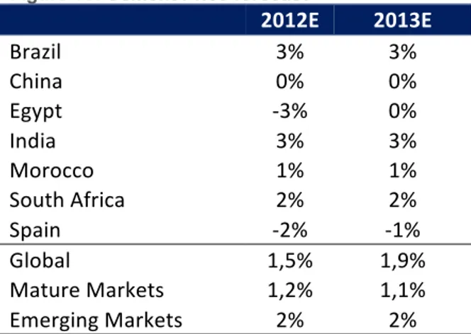
World cement consumption grew from 2782 million tons in 2008 to 3276 million tons in 2010, which corresponds to a cagr of 5,6%. In the figure below, it is possible to see the strong impact of the financial crisis in the most developed economies with American consumption decreasing 9% in 2009 and European 18%. The decrease of 9% in America is a result of a strong 24% decrease in North America. It is also important to highlight the performance of emerging economies which have been experiencing high growth rates namely China that grew about 38% between 2008 and 2010. Regarding future expectations, Credit Suisse analysts believe that cement industry will keep growing in the five regions.

China, 58,8% Others, 27,7%

India, 6,2% United States,