FACULDADE DE CIÊNCIAS
DEPARTAMENTO DE FÍSICA
NONLINEAR STATISTICS AND DYNAMICS
OF ATMOSPHERIC PREDICTABILITY
AND DOWNSCALING
Rui Alexandre Pita Perdigão
DOUTORAMENTO EM FÍSICA
FACULDADE DE CIÊNCIAS
DEPARTAMENTO DE FÍSICA
NONLINEAR STATISTICS AND DYNAMICS
OF ATMOSPHERIC PREDICTABILITY
AND DOWNSCALING
Rui Alexandre Pita Perdigão
DOUTORAMENTO EM FÍSICA
Tese orientada por:
Professor Doutor Carlos Alberto Leitão Pires
Doutor João Paulo da Costa Campos Teixeira
To begin with, I would like to express my deepest appreciation for the fundamental support provided by my thesis supervisor at the Univer-sidade de Lisboa, Prof. Doctor Carlos Alberto Leit˜ao Pires. In fact, as an ever-present guardian angel, Prof. Carlos Pires accompanied every stage of the research, even during my lengthy stay abroad.
I would also like to vehemently thank my supervisor at the NATO Un-dersea Research Centre (NURC), Doctor Jo˜ao Paulo da Costa Cam-pos Teixeira, for his hospitality and support, during the development of my research work at NURC under his supervision.
A word of utmost gratitude is due to Prof. Doctor Catherine Nico-lis and Doctor St´ephane Vannitsem, who openly welcomed me and supervised my research work at the Royal Meteorological Institute of Belgium (RMI). Even though I was at RMI as a visitor, I was pro-vided with excellent working conditions, namely an extremely inspiring scientific and human environment, along with ”royal” infrastructures.
My appreciation is extensive to all those whom I had the honour to interact with on a regular basis at the various institutions where the research work unfolded.
At the institutional level, I begin by acknowledging the crucial finan-cial support, throughout the whole doctoral period, from the Portuguese
Tecnologia, FCT), through the doctoral grant SFRH/BD/21471/2005, funded by the European Commission and the Portuguese Ministry for Science, Technology and Higher Studies (Minist´erio da Ciˆencia, Tecnologia e Ensino Superior). The thesis was elaborated under the auspices of the FCT-funded project PPCDT/CTE-ATM/62475/2004,
designated by PREDATOR − Seasonal Predictability and
Downsca-ling over the Euro-Atlantic Region.
Furthermore, I endoss my gratitude to the University of Lisbon (Uni-versidade de Lisboa) in general and the Instituto Dom Luiz (IDL) in particular, for being my academic home and behaving as such at all times, even during the years spent performing research work abroad.
Even though I have met just a handful of authors referred to through-out the thesis, I hereby express my gratitude to all of them for their remarkable and inspiring documents. In fact, the edifice of my work stands on the shoulders of giants.
I devote my final, kindest words of appreciation to my family. To them my whole self is owed... To them my whole work is dedicated...
This thesis addresses pertinent challenges underneath the estimation of the state of the system at a set of circumstances B given a set of conditions A. In particular, two main problems are considered: on one hand, that of atmospheric downscaling; on the other hand, that of atmospheric predictability.
For that purpose, novel methods in nonlinear statistics and dynamics are developed and implemented in the aforementioned contexts.
As far as the atmospheric downscaling is concerned, nonlinear statisti-cal features are assessed within the statististatisti-cal response of the monthly winter precipitation to the North Atlantic Oscillation (NAO) over the North Atlantic European Region. For that purpose, two major methodologies are developed and implemented.
On one hand, a diagnostic measure is built in order to measure the asymmetric part of an estimated variable’s response to its predictor, a measure undetected by linear correlation. As a practical application, that variable is chosen to be the precipitation and its predictor the NAO regime (NAO+ and NAO-). The asymmetric features are then used to define an asymmetry-based measure of non-Gaussianity.
On the other hand, an information-theoretical assessment on non-Gaussianity is performed and a corresponding measure of information-theoretical correlation − also transcending the limited scope of linear
correlation − defined and applied to the aforementioned downscaling application.
Gaussianity are proven to be consistent in their domain of validity. The statistical response of monthly precipitation to NAO is seen to be asymmetric and non-Gaussian. New relevant features are brought out as a result of the application of the proposed nonlinear statistical methods.
As far as atmospheric predictability is concerned, a systematic for-malism is derived for the dynamics of prediction errors under the combined influence of initial-condition and model-related errors. Its analytical results are confronted with those from numerical experi-ments and some generic features for the error dynamics are brought out and connected with intrinsic system properties.
Analytical and numerical results are seen to agree within the domain of validity of the analytical formulation: that of small perturbations in the short-to-intermediate time regime.
All in all, the proposed formulation for assessing the error dynamics is seen to allow for an evaluation of the dynamics of prediction errors without the need to actually run the numerical model under analy-sis. Moreover, it reveals new generic model-independent features of the error dynamics, under the combined influence of initial condition and model-related errors, not only for low-order but also to systems exhibiting a higher order of complexity.
A presente tese analisa desafios pertinentes subjacentes `a estima¸c˜ao do estado de um sistema num conjunto de circunstˆancias B dado um conjunto de condi¸c˜oes A. Em particular, dois problemas centrais s˜ao considerados: por um lado, o do ”downscaling” atmosf´erico; por outro, o da predictabilidade atmosf´erica.
Para tal, novos m´etodos em estat´ıstica e dinˆamica n˜ao lineares s˜ao desenvolvidos e implementados nos contextos acima referidos.
No que diz respeito ao ”downscaling” atmosf´erico, s˜ao analisadas ca-racter´ısticas estat´ısticas n˜ao-lineares da resposta estat´ıstica da pre-cipita¸c˜ao de Inverno `a Oscila¸c˜ao do Atlˆantico Norte (NAO) sobre a regi˜ao Euro-Atlˆantica. Para tal, s˜ao desenvolvidas e implementadas duas metodologias fundamentais:
Por um lado, ´e elaborada uma medida de diagn´ostico por forma a medir a parte assim´etrica da resposta de uma vari´avel estimada ao seu predictor, uma medida n˜ao detectada pela correla¸c˜ao linear. Como aplica¸c˜ao pr´atica, a vari´avel escolhida ´e a precipita¸c˜ao e o seu predic-tor o regime NAO (NAO+ ou NAO-). As caracter´ısticas assim´etricas s˜ao ent˜ao utilizadas para definir uma medida de n˜ao-Gaussianidade baseada na assimetria.
Por outro lado, a n˜ao-Gaussianidade ´e abordada na perspectiva da teoria da informa¸c˜ao, sendo definida uma medida de correla¸c˜ao baseada no conceito de informa¸c˜ao m´utua, transcendendo a correla¸c˜ao linear.
referido.
Como resultados principais, ´e provada a consistˆencia, no respectivo dom´ınio de validade, de estimadores propostos para a assimetria e n˜ao-Gaussianidade. Para al´em disso, ´e verificado que a resposta estat´ıstica da precipita¸c˜ao mensal `a NAO ´e assim´etrica e n˜ao-Gaussiana. S˜ao reveladas novas caracter´ısticas relevantes dessa resposta estat´ıstica em resultado da aplica¸c˜ao dos m´etodos estat´ısticos n˜ao-lineares pro-postos.
No que diz respeito `a predictabilidade atmosf´erica, ´e elaborado um formalismo sistem´atico para a dinˆamica dos erros de previs˜ao sob a influˆencia combinada de erros nas condi¸c˜oes iniciais e no pr´oprio modelo. Os seus resultados anal´ıticos s˜ao confrontados com os de ex-periˆencias num´ericas e s˜ao reveladas algumas caracter´ısticas gen´ericas, bem como a sua rela¸c˜ao com propriedades intr´ınsecas do sistema.
´
E verificada a concordˆancia entre os resultados anal´ıticos e num´ericos no dom´ınio de validade da formula¸c˜ao anal´ıtica: o das pequenas per-turba¸c˜oes no regime de prazos curtos a interm´edios.
No geral, verifica-se que a formula¸c˜ao proposta para analisar a dinˆamica do erro permite uma avalia¸c˜ao da dinˆamica dos erros de previs˜ao sem a necessidade de executar o modelo num´erico em an´alise. Para al´em disso, revela novas caracter´ısticas independentes do modelo em uso, sob a influˆencia combinada de erros nas condi¸c˜oes iniciais e no mo-delo, n˜ao s´o para sistemas de baixa ordem mas tamb´em para sistemas com mais elevado grau de complexidade.
Nonlinear Statistics; Atmospheric Downscaling; Non-Gaussianity; Information Theory.
Nonlinear Dynamics; Atmospheric Predictability; Error Dynamics; Chaos.
Palavras-chave
Estat´ıstica n˜ao-linear; ”Downscaling” Atmosf´erico; N˜ao-Gaussianidade; Teoria da Informa¸c˜ao.
Dinˆamica n˜ao-linear; Predictabilidade Atmosf´erica; Dinˆamica do Erro; Caos.
Acknowledgements iii Abstract v Resumo vii Keywords / Palavras-chave ix List of Figures xv Nomenclature xxvii 1 Introduction 1
2 Nonlinear statistical downscaling 7
2.1 Introduction . . . 7
2.2 Asymmetric correlation approach . . . 11
2.2.1 General correlation measures . . . 11
2.2.2 Asymmetric Gaussian correlations . . . 13
2.2.3 Measuring non-Gaussianity through asymmetric correlations 15 2.3 Information-theoretical approach . . . 17
2.3.1 Statistical Entropy . . . 17
2.3.2 Differential Entropy . . . 19
2.3.2.1 Definition . . . 19
2.3.3 Negentropy . . . 21
2.3.4 Relative Entropy . . . 22
2.3.5 Mutual Information . . . 24
2.3.6 Information Correlation . . . 26
2.4 Estimation of information-theoretical measures of non-Gaussianity 28 2.4.1 Edgeworth Expansion of a Bivariate Probability Density Function . . . 29
2.4.2 Application to non-Gaussianity estimation . . . 33
2.5 Dataset and processing . . . 35
2.5.1 Data . . . 35
2.5.2 Statistical Tests . . . 38
2.6 Results . . . 40
2.6.1 Gaussian and asymmetric correlations . . . 40
2.6.2 Cumulants and Edgeworth PDF applicability . . . 46
2.6.3 Mutual Information . . . 47
2.6.4 The Effect of Gaussian Anamorphosis . . . 51
2.7 Discussion and Conclusions . . . 53
3 Nonlinear Dynamics and Predictability 55 3.1 Nature of the problem . . . 55
3.1.1 The ’nemesis’ of atmospheric predictability . . . 56
3.2 An overview on Dynamical Systems . . . 57
3.3 Dynamics of prediction errors . . . 62
3.3.1 General formulation on a Hilbert space . . . 62
3.3.2 Error dynamics along Lyapunov vectors . . . 67
3.3.3 Short-term error dynamics . . . 68
3.3.3.2 Direct expansion . . . 74
3.3.4 Beyond Taylor expansions: a more robust analytical ap-proximation . . . 76
3.3.5 Short to intermediate time expansion in finite dimensional systems . . . 77
3.4 Error dynamics in illustrative systems . . . 86
3.4.1 Bistable systems . . . 86
3.4.2 Error dynamics around a saddle point . . . 92
3.4.3 Low order systems with chaotic dynamics . . . 97
3.4.3.1 The ”Lorenz (1963)” system . . . 97
3.4.3.2 A simple model for atmospheric circulation (Lorenz, 1984) . . . 105
3.4.3.3 A minimalist chaotic system (Rossler, 1976) . . . 111
3.5 Conclusions . . . 115
4 Error dynamics in a Quasi-Geostrophic model 117 4.1 Introduction . . . 117
4.2 Quasi-Geostrophic (QG) model . . . 118
4.3 Formulation on prediction errors for the QG model . . . 122
4.4 Analytical vs. numerical implementation . . . 126
4.4.1 Uniformly distributed perturbations in the initial condi-tions and constant ones in the parameters . . . 127
4.4.2 Anisotropic perturbations in the initial conditions and con-stant ones in the parameters . . . 133
4.4.3 Perturbations introduced at a particular scale of the motion 136
4.5 Sensitivity of the M.S.E. minimum to parameter error variations . 138
4.5.2 Perturbation in the initial condition and in the diffusive
time scale . . . 142
4.6 Probabilistic approach . . . 145
4.7 Discussion and Conclusions . . . 148
5 Beyond short-term − On a simple error model 153 5.1 Introduction . . . 153
5.2 Error growth model . . . 154
5.3 A Case study: the Quasi-Geostrophic model . . . 159
5.4 Discussion and Conclusions . . . 166
6 Conclusions 169
A Derivation of Eq. (2.11) 173
B Derivation of Eq. (2.47) 175
C Derivation of Eqs. (3.54)-(3.55) 177
D Derivation of Eq. (3.60) 179
E Proof of equivalence between Eqs. (3.50) and (3.59) 183
2.1 Skewness (a) and Kurtosis (b) of the distribution of monthly DJF
precipitation over the Euro-Atlantic area. . . 37
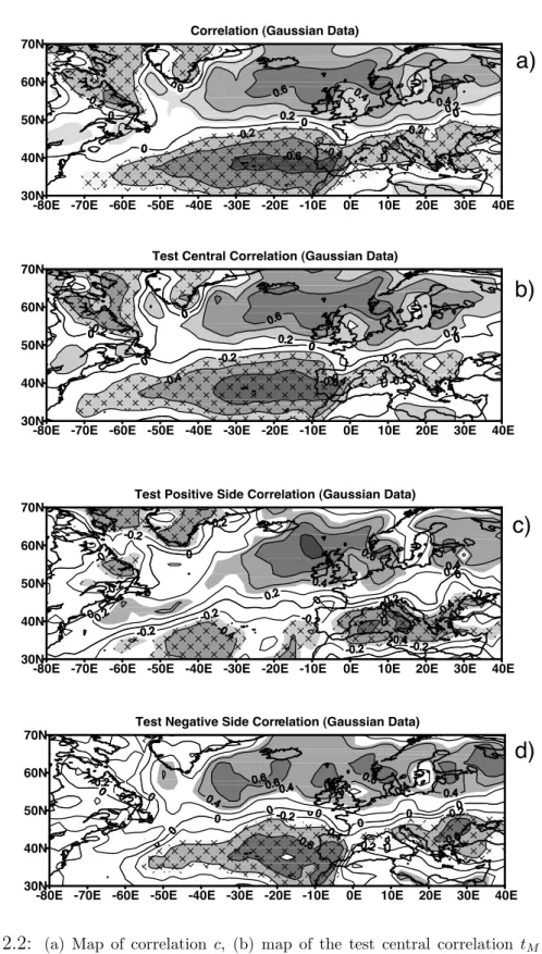
2.2 (a) Map of correlation c, (b) map of the test central correlation tM,
(c) map of the test positive side correlation t+, and (d) map of the
test negative side correlation t−. All quantities are computed for
Gaussian variables, i.e., subject to Gaussian anamorphosis.
Con-tour interval (CI) = 0.2. The significant regions (SR) at α = 90%
are shaded. The 90% significant area fractions FS-MCR are 0.73,
0.68, 0.44, and 0.44 for (a), (b), (c), and (d), respectively. Nearly
the same values hold for FS-MCG. . . 41
2.3 Composed graphics for the six selected points: (a) ATL, (b) BAL,
(c) EUS, (d) GRE, (e) SCO, and (f) RUS. Each graphic
con-tains 1) time series of the Gaussian precipitation (YG) against the
Gaussian NAO index (XG; filled circles for 1951−77, open circles
for 1978−2003); 2) contours of the corresponding joint PDF; and 3) linear and nonlinear prediction of YG. On top of each panel:
Smoothed graphics of the conditional RMSE of the linear (thin
2.4 (a) Map of the asymmetry Jc (CI = 0.02; SR at α = 90% shaded),
(b) map of the cumulant k(2,1) (CI = 0.1; SR at α = 90% shaded),
(c) map of the cumulant k(3,1) (CI = 0.1; SR at α = 90% shaded),
and (d) map of Pneg (CI = 0.002). All quantities computed are
subjected to Gaussian anamorphosis. The 90% significant area
fractions FS-MCR are 0.17, 0.17, and 0.19 for (a), (b), and (c),
respectively. Corresponding values of FS-MCG are 0.16, 0.13, and
0.15. . . 48
2.5 Map of the Gaussian mutual information Ig (CI = 0.1; SR at
α = 90% shaded), (b) map of the non-Gaussian MI (Edgeworth
estimator) (CI = 0.01; SF at 90% shaded), (c) map of the
informa-tion correlainforma-tion cinf. (CI = 0.1; SR at 90% shaded). All quantities
are computed for Gaussian variables. The 90% significant area
fractions FS-MCR are 0.73, 0.23, 0.22, and 0.64 for (a), (b), (c),
and (d), respectively. Corresponding values of FS-MCG are 0.73,
0.12, 015, and 0.57. . . 49
2.6 Non-Gaussian MI Ing(EF ) estimator as function of the ascending
order sorted values of non-Gaussian MI Ing(EI). . . . 50
2.7 (a) Map of the asymmetry test Jc for original data (CI = 0.02; SR
at α = 90% shaded), (b) Gaussian MI difference between Gaussian
and original data, (c) map of Pneg for original data. The 90%
sig-nificant area fractions FS-MCR is 0.17 for (a). The corresponding
3.1 Time evolution of the mean quadratic error in the presence of both
initial condition and model errors in the case of a bistable system
Eq. (3.64) with µ = 0.1. Initial condition errors are randomly
sampled from a uniform distribution around the steady state
so-lution of the exact system with "2 = 0.33× 10⁻⁶ and δµ = 10−3.
The full line depicts the exact solution, the dashed line the
lin-earised solution Eq. (3.67) and the dotted line the result of the
t-expansion. The number of realisations considered is 2× 10⁴. . . 89
3.2 As in Fig. 3.1 but for µ = 1. The dashed-dotted line stands for a
Pad´e approximant of the t-expansion [Eq. (3.52)]. . . 90
3.3 Time evolution and crossover time tc of the contributions of initial
condition and model errors (normalised by "2) considered
sepa-rately from the li-nearised expression (3.67) (full lines) and from
the t-expansion Eq. (3.69) (dashed lines) for the parameter values
of Fig. 3.1. . . 91
3.4 Time evolution of the mean quadratic error in the presence of both
initial condition and model errors around a saddle point. Full lines
stand for the exact expression (3.75a) and dotted lines for the
corresponding t-expansion (3.75b). Parameter values are " = δµ =
10−3, x
N = 1, λN = 1, µN = 0.1 (a), µN = 0.5 (b). . . . 95
3.5 As in Fig. 3.3 but for the saddle point case. Parameter values as
3.6 Short time behaviour of the mean square error, normalised by its
initial value, as obtained numerically (full lines) from model (3.68)
with r = 28 + δr, σ = 10, and b = 8/3 for three different values
of δr. Dashed lines stand for the Pad´e approximant [Eq. (3.52)]
of the corresponding third order analytic expansion [Eq. (3.62)].
Initial condition of the mean square error is!||u||2" ≡ !u2" = 10−6
and number of realisations for the averaging is 105. . . . 99
3.7 Crossover times, tc, of initial and model errors (dotted lines) for
two different magnitudes of error in the parameter r of the model
[Eq. (3.77)] as obtained from the corresponding analytic third
order t-expansion [Eq. (3.62)]. The other parameters are as in
Fig. 3.6. . . 100
3.8 Short to intermediate probability density of!u2"1/2 in the absence
of model error (full lines) and in the presence of model error, r =
28 + δr with δr = 5× 10⁻³ (dashed lines). Other parameters are
as in Fig. 3.6 and number of realisations is 106. . . . 102
3.9 Time when mean square errors attain their minimum, tm (a), and
relative size of the minimum (b), against the magnitude of the
model error perturbation δr. Full lines stand for the case of
unbi-ased initial condition errors and dashed lines for the case of biunbi-ased
ones. The amplitude of the bias is equal to the standard deviation
of the random part of the initial error of the variables of model
(3.77). Parameters are as in Fig. 3.6 and number of realisations is
3.10 Short-to-intermediate time behaviour of the mean square error,
normalised by its initial value, as obtained numerically (full lines)
from model (3.81) with a = 0.25, b = 4, F = 8, G = 0.9 for three
different values of δG: a) δG = 0.04; b) δG = 0.02; c) δG = 0.
Dashed lines stand for the Pad´e approximant [Eq. (3.52)] of the
corresponding third order analytic expansion [Eq. (3.62)]. Initial
condition of the mean square error is !||u||2" ≡ !u2" = 10−6 and
number of realisations for the averaging is 104. . . . 108
3.11 Time evolution of the mean square error, normalised by 10−6, of
the analytical approximation to the model (3.81) with a = 0.25,
b = 4, F = 8, G = 0.9, for a case in which only errors in the
initial conditions are considered: !u2" = 10−6 and δG = 0 (full
line); and three scenarios without errors in the initial conditions:
!u2" = 0 and δG = 0.02 (dotted line), δG = 0.04 (dashed line)
and δG = 0.06 (dashed-dotted line). Crossovers occur when the
error curve stemming from model errors crosses that from errors
in the initial conditions (tc ≈ 0.175 for δG = 0.06, tc ≈ 0.3 for
δG = 0.04). The number of realisations considered in the averaging
3.12 Short-to-intermediate time behaviour of the mean square error,
normalised by its initial value, as obtained numerically (full lines)
from model (3.84) with a = b = 0.2, c = 5.7 for three different
val-ues of δc: a) δc = 0.018; b) δc = 0.012; c) δc = 0.006. Dashed lines
stand for the Pad´e approximant [Eq. (3.52)] of the corresponding
third order analytic expansion [Eq. (3.62)]. Initial condition of
the mean square error is !||u||2" ≡ !u2" = 10−6 and number of
realisations for the averaging is 104. . . . 112
3.13 Time evolution of the mean square error, normalised by 10−6, of
the analytical approximation to the model (3.84) with a = b = 0.2,
c = 5.7, for a case in which only errors in the initial conditions are
considered: !u2" = 10−6 and δc = 0 (full line); and three scenarios
without errors in the initial conditions: !u2" = 0 and δc = 0.006
(dotted line), δc = 0.012 (dashed line) and δc = 0.018
(dashed-dotted line). Crossovers occur when the error curve stemming
from model errors crosses that from errors in the initial conditions
(tc ≈ 0.018 for δc = 0.018, tc ≈ 0.027 for δc = 0.012 and tc ≈ 0.055
for δc = 0.006). The time is presented in logarithmic scale and the
4.1 Forecasting-time evolution of the mean quadratic error of the
hor-izontal velocity (zonal and meridional), normalised relative to its
initial value and averaged over the whole spectrum and levels, in
the presence of uniformly distributed initial condition errors with
variance 10−6m2s−2 and with the addition of error in the forcing
term |δS| = 0.02, with the Kinetic Energy metric over the sphere.
The number of realisations considered in the process is 5000. . . 129
4.2 Same as Fig. 4.1, but considering error in the diffusion time
|δτDIF| ≡| dTDIF| = 0.2, instead of that in the forcing term. . . 129
4.3 Forecasting-time evolution of the mean quadratic error of the
hor-izontal velocity (zonal and meridional), normalised relative to " =
10−6m2s−2 and averaged over the whole spectrum and levels, with
the Kinetic Energy metric over the sphere. The full line represents
the case considering the presence of uniformly distributed initial
condition errors with variance " and no model error, whereas three
model-imperfect scenarios are considered in the absence of errors in
the initial conditions: δS = 0.02 (dotted line), δS = 0.04 (dashed
line) and δS = 0.06 (dashed-dotted line). The number of
real-isations considered in the averaging over an ensemble of initial
4.4 Forecasting-time evolution of the mean square error of the
hori-zontal velocity (zonal and meridional), normalised relative to its
initial value and averaged over the whole spectrum and levels, in
the presence of uniformly distributed initial condition errors with
variance 10−6m2s−2 subsequently subjected to breeding, with the
addition of error in the forcing term |δS| = 0.02 and with the
Ki-netic Energy metric over the sphere. The number of realisations
considered in the process is 5000. Three cases are considered:
with-out breeding (BT=0) and with breeding times BT of 24 h and 72
h. . . 135
4.5 Forecasting-time evolution of the mean square error of the
horizon-tal velocity (zonal and meridional), normalised relative to its
ini-tial value and averaged over the three levels, in the presence of
uni-formly distributed initial condition errors with variance 10−6m2s−2
and with the addition of error in the forcing term|δS| = 0.02, with the Kinetic Energy metric over the sphere. The number of
realisa-tions considered in the process is 5000. Three total wavenumbers
representing small (n = 20), intermediate (n = 11) and large scales
4.6 Time at which the mean square error of the horizontal velocity
(zonal and meridional) is minimum, for different values of the error
in the forcing term, in a Quasi-Geostrophic model [Eq. (4.1)]. The
triangles refer to the case in which there is a systematic error of
1× 10⁻⁶m2s−2 in the initial conditions. The squares refer to the
case in which the initial condition errors are random, uniformly
distributed as in Fig. 4.1. The circles refer to the case in which
both systematic and random initial condition errors are considered.
The number of realisations and the metric used for averaging are
as in Fig 4.1. . . 139
4.7 Normalised minima of the mean square error of the horizontal
ve-locity (zonal and meridional) for different forcing errors, as in Fig.
4.6, in the following cases: (a) systematic error of 1× 10⁻⁶m2s−2
in the initial conditions; (b) random, uniformly distributed initial
condition errors as in Fig 4.1; (c) both systematic and random
initial condition errors are considered. The normalisation factor is
4.8 Time at which the mean square error of the horizontal velocity
(zonal and meridional) is minimum, for different values of the error
in the diffusive term τDIF in a Quasi-Geostrophic model [Eq. (4.1)].
The triangles refer to the case in which there is a systematic error
of 1× 10⁻⁶m2s−2 in the initial conditions. The squares refer to the
case in which the initial condition errors are random, uniformly
distributed as in Fig4.1. The circles refer to the case in which both
systematic and random initial condition errors are considered. The
number of realisations and the metric used for averaging are as in
Fig4.1. . . 143
4.9 Normalised minima of the mean square error of the horizontal
ve-locity (zonal and meridional) for different errors in the diffusive
term τDIF (days), as in Fig. 4.8, in the following cases: (a)
sys-tematic error of 1×10⁻⁶m2s−2in the initial conditions; (b) random,
uniformly distributed initial condition errors as in Fig4.1; (c) both
systematic and random initial condition errors are considered. The
normalisation factor is 1× 10⁻⁵. . . . 144
4.10 Short to intermediate time statistical distribution of the mean
square error in horizontal velocity (zonal and meridional),
nor-malised with respect to that of its initial distribution, in the
ab-sence (a) and in the preab-sence (b) of model error, |δS| = 0.04. The
number of realisations considered in the averaging over the
5.1 Time evolution of the base 10 logarithm of the L2 norm error in
the non-dimensional Streamfunction state vector of the QG model
based on the difference between numerical results with time steps
∆t of 180, 80, 40, 20, 10, 5 and 2.5 minutes and those obtained
with the control time-step of 1.25 minutes. . . 160
5.2 Representation of Fig. 5.1using our proposed error growth model.
The chosen parameters are λI = 0.5, η = 4, α = 0.2, β = 0.01,
σd = 0.01, "∆t = 10−12(∆t)4, "u0 = 0, "s0 = 0, where ∆t, the time
steps considered, are the same as those in Fig. 5.1. . . 160
5.3 Time evolution of the base 10 logarithm of the L2 norm error in
the non-dimensional Streamfunction state vector of the QG model
based on the difference between numerical results with time step
∆t of 10 minutes and those obtained with the control time-step of
1.25 minutes (numerical solution, represented in circles).
Repre-sentation of the numerical solution using our proposed error growth
model [Eqs. (5.3a), (5.3b)] (solid line), with parameters as in Fig.
5.2. Best fit of the Savijarvi (1995) model [Eq. (5.6)] with respect
to the numerical solution (crosses). . . 163
5.4 QG actual model run case as in Fig. 5.1: Time-evolution of the
ratios between the logarithms of the simulated error in the unstable
directions, for the following time steps (B vs. A): 80 min vs. 40
min, 40 min vs. 20 min, 20 min vs. 10 min, 10 min vs. 5 min, 5
5.5 QG case as simulated with the proposed error growth model as in Fig. 5.2: Time-evolution of the ratios between the logarithms of the simulated error in the unstable directions, for the following time steps (B vs. A): 80 min vs. 40 min, 40 min vs. 20 min, 20 min vs. 10 min, 10 min vs. 5 min, 5 min vs. 2.5 min. . . 165
Roman Symbols
A Self-adjoint operator defined semi-positive
B Positive-defined operator
c+ Positive side correlation, i.e. correlation between two variables X and Y
conditioned to X being above its median MX
c− Negative side correlation, i.e. correlation between two variables X and Y conditioned to X being above its median MX
cg Gaussian Correlation
cinf Information Correlation
cM Interset Covariance or Central Correlation
C Covariance operator
c(X, Y ) Pearson Correlation between variables X and Y
d Integral term due to model error or drift
D Dissipative term in the QG model
E Ekman term in the QG model
exp Exponential function, exp(a) = ea
E(.) Expectancy
EZ+ Conditional Expectancy of generic variable Z given data above the median
EZ− Conditional Expectancy of generic variable Z given data below the median
F Smooth function representing a dynamical system
f generic nonlinear function
f Model formulation, smooth nonlinear function with continuous derivatives over the whole domain
F H(h) Dependency of the drag coefficient on height h g generic nonlinear function
G Gaussian Anamorphosis
h Height
H(.) Statistical Entropy h(.) Differential Entropy
Hi Hermite orthogonal polynomials of order i
H Hilbert space
Ho Null hypothesis
Ig Mutual Information within the bivariate Gaussian distribution with
corre-lation c
Ing Mutual Information term associated to non-Gaussianity
Ing(EF ) Estimation of the Mutual Information term associated to non-Gaussianity
from the Edgeworth expansion method
Ing(EI) Mutual Information term associated to non-Gaussianity obtained through
an estimated integral
Ing(M I) Estimation of the Mutual Information term associated to non-Gaussianity
by Gaussian quadrature
% Imaginary part of the term onto which it operates I Interval withinR
I Mutual Information
J Jacobian of the model relative to the state vector
J Negentropy
Jc Asymmetry measure
Jl l-th order time derivative of J
Js Jacobian of the 2D field over the sphere
J(V, W ) Joint Negentropy of V and W
KJ Operator defined by M−1JM
δkr
k(p,q) Cumulants of order p in V and of order q in W
kur Kurtosis
l Positive adimensional quantity increasing with the truncation order (ex-cept when used as a generic subscript)
ln Natural logarithm, i.e. loge(.)
LS(λ, φ) Fraction of land within a grid box n the QG model
M Fundamental (resolvent) matrix
M Median
n Generic non-negative integer, n∈ N0
N (·) Norm
Ndf Number of temporal degrees of freedom
neq Number of i.i.d. variables
N L Number of levels considered in the spectral mode
N T Truncation of a spectral model
O Generalised self-adjoint Oseledec operator
Ol l-th order time derivative of O at forecast time τ = 0
O(i) i-th order term
P Pad´e Approximant
Pneg Integral of the EDG-PDF in the domain of negative values of the estimated
Ppos Integral of the EDG-PDF in the domain of positive values of the estimated
truncated density
p Probability function
p Tendency error
pT Pressure on top of the troposphere
pX(x) Probability that X = x
P (X = x) Probability that X = x
q Potential Vorticity
Q Generic Quantile
' Real part of the term onto which it operates R Real set
rE Average radius of the Earth
rhs Right hand side
Rj Rossby radii of deformation in the QG model
S Forcing term in the QG model
sgn(·) Signal of a function
t Time
Ti Coefficient of the τi term in the Taylor expansion in τ
t− Test Negative Side Correlation
tc Crossover time, for which the magnitudes of the contributions of initial
and model errors match each other
tM Test Central Correlation
tm Time at which the mean square errors attain their minimum value
T Transpose (as superscript)
u Error in the state vector
u0 Error in the initial conditions, i.e. of the state vector at time t = 0
uI Integral term due to error in the initial conditions
V Standard variable assumed as arithmetic average of neq independent and
identically distributed (i.i.d.) variables.
var Variance
W Standard variable assumed as arithmetic average of neq independent and
identically distributed (i.i.d.) variables.
wi Weighing term representing the metric defined on an orthogonal basis
x State vector of a dynamical system
X Generic variable with values x∈ R X Generic n-dimensional variable
XG Gaussian random variable with the same covariance matrix as that of X
Y Generic variable with values y ∈ R
Yr Standardised residue of the linear prediction of Y from X
Z Generic variable with values z∈ R
Z Generic operator
Greek Symbols
" Isotropically distributed errors in the initial conditions
"∆t One-step integration error given the time-step ∆t
"s Error in the direction of the stable modes
"u Error in the direction of the unstable modes
ηαt"" Eigenvalues of O (real-valued)
Γ Actual phase trajectory
ΓR Reference phase trajectory
λαt"" Finite Lyapunov exponent between times t"" and τ
Λα,t"" Set of finite Lyapunov vectors optimised between times t"" and τ , α being
the index referring to each vector
λI Sensitivity to the initial conditions
λx0 Lyapunov exponents
µ Control parameters of a dynamical system
ν Truncated fitting polynomial vanishing if the joint PDF is Gaussian
Ω Alphabet of a random variable
Φ Jacobian of the model (f ) relative to the control parameters
Φl l-th order time derivative of Φ
Φ Cumulative standard Gaussian distribution function
φα Orthonormalisation vector
ϕ Standard Gaussian PDF
ϕV(v) Marginal Probability Distribution Function of V
Π Projection operator over a sub-space of the basis functions φα
Ψ Streamfunction
ρ Probability Density Function
ρV,W(v, w) Joint Probability Distribution Function of V and W
σ Standard Deviation
σd Rate of decay of stable modes
σZ+ Conditional Standard Deviation of the generic variable A given data above the median of Z
σZ− Conditional Standard Deviation of the generic variable A given data below
the median of Z
τDIF Diffusive time scale in the QG model
τR Radiative time scale in the QG model
ξp Potential Vorticity in the pressure coordinate system
Other Symbols
∗ Complex conjugate (as superscript) !· · ·" Phase space average over the attractor
δf Deviation of the model formulation relative to the true dynamics it indends to represent
δµ Error in the control parameters
∆p Pressure difference between levels in the QG model
δΨ Perturbation in the Streamfunction
δq Perturbation in the Potential Vorticity
∆t Time-step
δSST Sea surface temperature anomaly with respect to the climatology )·, ·* Inner product
#
2D gradient operator over the sphere
· · · Average over an ensemble of initial conditions
→ Tends towards
Acronyms
2D Bidimensional
4D-Var Four-dimensional variational data assimilation
ATL Central Atlantic
BAL Balearic Islands
BT Breeding time
DJF December to February
ECMWF European Centre for Medium-Range Weather Forecasts
EDG Edgeworth expansion
EDG-PDF Probability Distribution Function estimated through an Edgeworth expansion
EUS Eastern United States
FCT Funda¸c˜ao para a Ciˆencia e Tecnologia
FS Fraction of statistically significant area
FS-MCG Fraction of statistically significant area for the MCG method
FS-MCR Fraction of statistically significant area for the MCR method
GA Gaussian Anamorphosis
GRE Greenland
ICA Independent Component Analysis
IDL Instituto Dom Luiz
i.i.d. Independent and identically distributed
KLD Kullback-Leibler Distance
L3 Three-level
MCG Monte Carlo technique through generation of Gaussian noise
MCR Monte Carlo technique through random reordering of working series
MI Mutual Information
NAE North Atlantic European Region
NAO+ Positive phase of the North Atlantic Oscillation
NAO- Negative phase of the North Atlantic Oscillation
NAO North Atlantic Oscillation
NATO North Atlantic Treaty Organisation
NCEP/NCAR National Centers for Environmental Prediction− National Center
for Atmospheric Research
NURC NATO Undersea Research Centre
PDF Probability Density Function
QG Quasi-Geostrophic
RMI Royal Meteorological Institute of Belgium
RUS Russia
SCO Northwest Scotland
SLP Sea level pressure
SR Significant Regions
SST Sea surface temperature
Introduction
A fundamental challenge driving scientific work consists on finding a solution for a problem given a set of available factors. For that purpose, adequate metho-dologies have to be developed and implemented that somehow allow for the factors to weigh in, providing input that will help drive the problem towards a solution.
In physical sciences, given the state of a system under a certain set of cir-cumstances (say, A), quantitative methods can be elaborated and used for its estimation at another set of circumstances, say B. By circumstances it is meant, for instance, a series of equations, inequalities, probabilities of events, all ex-pressed in terms of the set of variables characterising the state of the system.
When B positions the system at a future state relative to A, its estimation is commonly denoted as prediction. The aforementioned quantitative methods take the form of a model representation also denoted as prediction system.
There are, however, major obstacles in achieving reasonable skill in such esti-mation. On one hand, there are uncertainties in the input factors, stemming from the limited accuracy of their measurement and assessment. In highly unstable systems, even the slightest inaccuracy way below the resolution limits of the most advanced measurement equipment at hand can ultimately contribute to an utter
loss of predictability. This rather surprising fact is a core signature of chaos, in the sense of sensitive dependence to prior conditions (Lorenz, 1963).
On the other hand, the prediction system itself does not encompass the full
extent of the physics involved in the process. In fact, there are physical rela-tionships and additional factors not taken into account, such as sub-grid scale processes and errors in the model formulation itself. This, too, can seriously undermine the predictive ability.
These issues are of utmost relevance for the atmospheric sciences. In fact, at-mospheric prediction systems are known to suffer from fundamental uncertainties associated with their sensitivity to the initial conditions and with the inaccuracy in the model representation. The idea that error in weather forecasting comes from both these sources of uncertainty can be traced back to as early asBjerknes
et al. (1911).
Initial condition uncertainties and their role in affecting the predictability have been widely studied for a long time, e.g. as early as Thompson (1957), Lorenz
(1963). This error source was addressed both in the context of dynamical systems predictability (e.g. Lorenz, 1963; Smith et al., 1999) and ensemble forecasting (e.g. Nicolis, 1992; Toth and Kalnay, 1993; Nicolis et al., 1995, Buizza and
Palmer, 1998).
More recently model errors have been addressed both at the level of numerical forecast models (e.g. Dalcher and Kalnay, 1987; Reynolds et al., 1994) and their generic features (Vannitsem and Toth,2002;Nicolis,2003,2004). Moreover, their connections with such error sources in numerical truncation (e.g. Teixeira et al.,
2007) sub-grid scale parameterisations (e.g. Teixeira and Reynolds,2008; Buizza
ever, by solely focusing on one of these error types only limited improvement in prediction can be attained (Lorenz, 2005). Moreover, the combination of these factors is known to place severe limits on our ability to predict future states of even thoroughly-understood systems. It is thus of interest to study the dynamics in the presence of both error types in a systematic manner. This was one of the main objectives of the present thesis.
For this purpose, methods in nonlinear dynamics were developed, tested and implemented that allowed for generic and relevant case-by-case features to be brought out in systems relevant to the physical sciences in general and the atmo-spheric sciences in particular. In this context, the theoretical developments and their applications to illustrative systems are presented in chapter 3, followed by an implementation in a Quasi-Geostrophic (QG) model (Marshall and Molteni,
1993) in chapter 4.
Chapter 3 begins with an overview on dynamical systems and predictability, followed by the general framework on the dynamics of model error in a generic, indimensional functional space. The formulation is then simplified to finite-dimensional systems, envisioning the practical applications to be presented after-wards. Some generic, model-independent features are brought out, such as the role of the mechanisms of error transfer between a particular initial direction to components along other directions, the existence of a minimum in the error evo-lution and the relative importance of the IC errors and model errors in the global evolution. These theoretical results are then tested and illustrated in low-order systems exhibiting bistable, saddle-point and chaotic behaviour.
In chapter4the generic analytical approach to the error dynamics introduced in3is applied to the QG model and validated with numerical experiments. While
some generic features are identified that come in agreement with those seen in lower-order systems, further properties of physical relevance, stemming from the higher-order of complexity of the system, are also unveiled.
A rather different approach to the error dynamics in a QG model from that of the preceding chapters is then presented in chapter 5. There, a simple model of error evolution is presented by considering the relative error growth rates in the stable and unstable directions, with the addition, in the latter case, of a nonlinear saturation term that allows for the error evolution to be modelled on the long term until saturation.
Another major objective brings us back to challenges underneath the estima-tion of the state of the system at B given A, though in a different context: that of atmospheric downscaling, in which local or regional-scale atmospheric features are inferred from large-scale atmospheric predictor variables.
In this context, while a dynamical approach would be a natural favourite from a physical point of view, there is no conclusive evidence that dynamics should be favoured over statistics. In fact, by comparing these approaches overall similar skills can be obtained, with statistical methods coming out on top when it comes to such practical aspects as computational effort (Murphy, 1999; Kidson and
Thompson, 1998). Anyway, regardless of the methodology one must never lose
sight of the underlying physical phenomenology.
The scientific literature exhibits a wealth of relevant work on atmospheric downscaling, most notably on extracting such features as regional circulation, temperature and precipitation regimes from large-scale patterns in the climatic system such as the North Atlantic Oscillation (NAO) (e.g. Trigo et al.,2002,2004;
Pires and Perdig˜ao, 2007) or the El Ni˜no / Southern Oscillation (ENSO) (e.g.
statistical methods that significantly increase the quality of the estimation, along with relevant examples of application.
In the present thesis, nonlinear statistical features are assessed within the sta-tistical response of the monthly winter (December to February) precipitation to the North-Atlantic Oscillation (NAO) over the North Atlantic European Region (NAE). For that purpose, two major methodologies are developed and imple-mented:
On one hand, a diagnostic measure is built in order to measure the asymmetric part of an estimated variable’s response to its predictor, a measure undetected by linear correlation. As a practical application, that variable is chosen to be the precipitation and a certain predictor: here, the NAO index, splitting the NAO+ and NAO- regimes. The asymmetry is based on the different anti-symmetric responses to NAO+ and NAO-. The asymmetric features are then used to define an asymmetry-based measure of non-Gaussianity.
On the other hand, an information-theoretical assessment on non-Gaussianity is also performed and a corresponding measure of information-theoretical corre-lation − also transcending the limited scope of linear correlation − defined and
applied to the aforementioned downscaling application.
This key objective encompassing nonlinear statistics and downscaling is tho-roughly addressed in chapter 2, as it chronologically preceded the work on non-linear dynamics and predictability (chapters 3− 5), from which it is technically independent.
While each chapter has its own conclusions, the thesis is concluded with a closure chapter with final, concluding remarks and future prospects (chapter 6).
Nonlinear statistical downscaling
2.1
Introduction
The characterisation of large-scale extratropical atmospheric variability is a matter of open debate. A paradigmatic view is to regard the low-frequency projection of the atmospheric attractor as a superposition of dynamical regimes (Dole, 1983).
It has been suggested and argued that atmospheric large scale variability at the monthly time scale over the North Atlantic European Region (NAE) is characterised by transition or permanence among four dynamical winter regimes: the positive phase of the North Atlantic Oscillation (NAO+), its negative phase (NAO-), the Greenland-Scandinavian dipole (GS) and the Atlantic anticyclonic ridge (RDG) (Cassou et al., 2004). These regimes, obtained by cluster analy-sis, are not exactly organised symmetrically around the climatology, in terms of symmetry relative to axis of uncorrelated variables. In fact, they are asymme-tric, as it normally occurs in chaotic nonlinearly forced systems (Palmer, 1999). Moreover, composites of anomaly surface forcings [e.g. sea surface tempera-ture (SST)], computed for opposite regimes, show some degree of asymmetry
expectan-cies: E(δSST|NAO+) ,= −E(δSST|NAO-), where δSST is the SST anomaly
with respect to the climatology. This has been shown in particular for the tripole Atlantic and Pacific SST forcings of the NAO+ and the NAO- quasi anti-symmetric regimes (Cassou et al., 2004). The link between average surface climatic conditions (e.g. large-scale precipitation and surface temperature) and middle-tropospheric regimes can be decomposed in terms of a monotonic line-ar influence and nonlineline-ar terms responsible for possible asymmetric responses. A linear response of the mean square error (MSE) to a forcing is a necessary, though not sufficient condition of joint Gaussianity between the response and forcing. Therefore, a nonlinear MSE-response implies non-Gaussianity. As a con-sequence, the joint probability density functions (PDFs) of large-scale indexes and climatic variables can express some degree of asymmetry and non-Gaussianity. Some studies corroborate this fact, e.g. the nonlinear, asymmetric response of the surface temperature over Europe for symmetric quantiles of the North At-lantic Oscillation (NAO) index (Pozo-V´asquez et al., 2001; Trigo and Palutikof,
1999). Another example is the asymmetry of dry and wet Self-Organizing Maps
(Cavazos,2000) and their different correlations with Arctic Oscillation and NAO
indices. Another study hypothesises the asymmetric response of the Indian Ocean precipitation to the NAO (Sapiano and Arkin personal communication, 2005).
Motivated by this issue, we hereby bring a contribution to inferring the degree of non-Gaussianity and asymmetry within the statistical response of the monthly winter [December−February (DJF)] precipitation to the NAO over the NAE.
Both the mean influence of NAO and its trend on the monthly winter precipi-tation over the NAE are well documented (Hurrell et al., 2004). That influence is essentially due to: a) the different tracking of synoptic storms in the presence of NAO+ or NAO- regimes (Rogers, 2002; Hurrell, 1995); b) the enhancement,
for particular regimes, of local systems associated to particular geographical and orographic conditions, for instance for Greenland and Iceland (Serreze et al.,
1997).
The linear component of that influence can be assessed through the one point linear correlation map between the monthly precipitation and the NAO monthly index, which is defined as the Lisbon, Portugal, minus Stykkisholmur, Iceland, normalised average monthly sea level pressure (SLP) anomaly or other correlated quantities (Osborn et al.,1999). In practice one begins by computing a quantity A given by the normalised monthly anomaly at Lisbon minus the normalised monthly anomaly in Iceland. Then the NAO index is obtained by normalising A. The aforementioned correlation map shows a dipolar structure with extreme positive correlations near 0.6, at south of Iceland, around 60oN latitude, and
extreme negative values near −0.6 at the North Atlantic basin around 40oN of
latitude.
A diagnostic measure is hereby built in order to measure the asymmetric part of the precipitation response to NAO, undetected by the linear correlation. For that purpose, side or asymmetric correlations between NAO index and monthly precipitation are computed. This essentially consists of evaluating conditional correlations for both the positive and negative NAO regimes, thus revealing pos-sible asymmetric or non-Gaussian precipitation responses to NAO. Asymmetry is only a particular aspect of something more general: non-Gaussianity.
The Edgeworth expansion method is used to evaluate bivariate non-Gaussian probability densities (PDFs). Then, relevant diagnostics are obtained from Infor-mation Theory (Shannon, 1948), such as Negentropy and Mutual Information as well as its Gaussian and non-Gaussian counterparts (Kraskov et al.,2004). This method assumes a weak non-Gaussianity scenario. The non-Gaussianity degree
of the joint PDF (NAO, Monthly Precipitation at the point basis) is evaluated
through Edgeworth Expansions (Edgeworth, 1905; Comon, 1994), based on the
Hermite Polynomials (Abramowitz and Stegun,1972) and higher-order statistical
moments.
PDF evaluation is also possible numerically based in the Maximum Entropy
Principle (Pires and Perdig˜ao,2007;Jaynes, 1982), through the Maximum
Like-lihood Method (Sivia, 1996) and the Kernels estimation (Silverman, 1986).
Apart from the present document, Information Theory is used in other
appli-cations such as predictability studies (DelSole, 2004), forecast evaluation (
Roul-ston and Smith,2002), Independent Component Analysis (ICA) of climatological
data (Aires et al., 2002; Perdig˜ao, 2004), computation of Mutual Information
among climatic data (Marwan and Kurths,2002;Perdig˜ao, 2004).
In the upcoming sections a theoretical overview is presented on the asymmetric
correlation (section 2.2) and information-theoretical concepts (section 2.3)
rele-vant for the problem. Methodologies for the estimation of information-theoretical
measures of non-Gaussianity are presented in section 2.4. Data and processing
methodologies are then presented (section2.5), followed by results and their
anal-ysis (section2.6). The chapter is then concluded with a final discussion (section
2.7).
The new developments presented in this chapter have been included in the
research paper byPires and Perdig˜ao (2007), published in the Monthly Weather
2.2
Asymmetric correlation approach
2.2.1
General correlation measures
Let us begin by recalling the widely used Pearson Product-Moment Corre-lation Coefficient, also known as Pearson CorreCorre-lation (Papoulis, 1991). It is a measure of the degree of linear relationship between two variables X and Y , given by
c(X, Y ) = E[X!− E(X)]E[Y − E(Y )]
var(X) var(Y ) (2.1)
where var(X) = E[(X− E(X))2].
While practical in most applications, this measure does not account for the overall statistical dependence between variables − nonlinear relationships are left unaccounted for. In fact, it is possible to have such dependence even when
c(X, Y ) = 0.
In order to illustrate this fact, consider a uniformly distributed random vari-able with values x ∈ [0, 2π[. Consider now two nonlinear functions, f(x) = sin(x) and g(x) = cos(x). These are clearly dependent from each other; in fact,
g(x) = f (|x + π/2|) for all x in [0, 2π[. However, it can easily be seen that
c[f (x); g(x)] = 0, ∀x ∈ R. One is thus led to the conclusion that null Pearson
correlations do not imply statistical independence.
Anyway, one must note that, while not a sufficient condition for independence, a null Pearson correlation is a necessary condition for that purpose. In fact,
c(X, Y ),= 0 implies statistical dependence between the intervening variables.
Even though c(X, Y ) ,= 0 does not take into account nonlinear relationships between the intervening variables, it is possible to peer into such relationships by considering the Pearson correlation between general nonlinear functions f (X) and g(Y ): c(f (X); g(Y )). When f (X) = E(Y|X = x) and g(Y ) = E(X|Y = y)
these relationships are maximised in absolute value. This is a way of using the linear, Pearson correlation to define nonlinear correlations.
A particular example of nonlinear correlation measure is the Spearman or rank correlation (Wilks,1995), where the nonlinear functions are simply the sampling ranks of X and Y respectively. These ranks measure the degree of monotonic association between both variables.
Another nonlinear correlation measure can be defined by taking, as nonlinear functions f and g, the standard Gaussian transformation or Gaussian
Anamor-phosis of the original variables (Wackernagel, 2003). It is hereby denoted as
Gaussian Correlation and defined as:
cg = c(GX; GY) (2.2)
where GX (equivalently for Y ) is the Gaussian Anamorphosis of X, given by:
GX(x) = Φ−1 "# x −∞ ρX(u) du $ , (2.3)
where ρX(u) is the probability density function of X and Φ−1 is the inverse of the
cumulative standard Gaussian distribution function.
This transformation is a common data analysis procedure in geostatistical kriging and climatic data analysis (Biau et al., 1999) that ensures that the marginal distributions are standardised Gaussian.
Since the correlation in (2.2) relates two Gaussian variables, GX and GY, it
is an optimal measure of their dependence, as Gaussian variables only exhibit linear statistical dependence. One must, however, note that while the marginal distributions are standard Gaussian, their joint distribution is not necessarily Gaussian. In the particular case for which X and Y are Gaussian, cg(X, Y ) =
Both rank and Gaussian correlations are nonlinear correlations invariant for the class of monotonous homeomorphisms on X and Y individually (though not necessarily homeomorphisms mixing these variables). Consequently, an advan-tage of both these measures over the Pearson correlation is the fact that, unlike the latter, the formers are not artificially inflated by the coincidence of large outlier values (Jolliffe and Stephenson,2003).
2.2.2
Asymmetric Gaussian correlations
The correlation measures presented in the previous section take into account the statistical sensitivity of variables to one another in their domain as a whole. However, their statistical relationships within a particular subdomain are not accountable by such general measures. In order to overcome this limitation, we refer to the concept of Asymmetric Correlation (Pires and Perdig˜ao, 2007). It consists on the conditional correlation between two standard variables X, Y for a certain interval IX of X, represented by c(X, Y|X) ∈ IX. The asymmetric
correlation measure is particularly relevant when the sensitivity of one variable
Y to another X is not necessarily the same over every subdomain of X.
A simple partition of X can be considered into two complementary intervals, separated by a quantile QX of X. Within this context, a particular case can be
taken for the QX = MX, the latter being the median of X. In this case, the two
partitions are equally-sized.
The correlations between two variables X and Y conditioned to X being below and above its median MX are then given, respectively, by:
c+= c(X, Y|X > MX)
c−= c(X, Y|X < MX)
and the conditional standard deviations, for each half of the data: σZ+ = [var(Z|X > MX)] 1/2 σZ− = [var(Z|X < MX)] 1/2, Z = X or Y, (2.5)
where var denotes variance.
By considering X and Y to be centred and to have unit-variance, their ex-pectation values within each of X’s considered subdomains relate to each other in the following way:
E(Z|X < MX) =−E(Z|X > MX),
Z = X or Y
(2.6)
For simplicity of notation, let E(Z|X < MX)≡ EZ− and E(Z|X > MX)≡ EZ+. Under the same conditions − X and Y centred and with unit-variance − the
following relation is also held:
1 = (EZ+) 2+1 2 % σ2Z− + σZ2+ & , Z = X or Y (2.7)
A nonlinear asymmetric relationship between X and Y can be assessed through differences between the asymmetric correlations c+ and c− in (2.4). For standard
variables the correlation equals the covariance, which can be decomposed into
intra- and interset covariances.
By taking the aforementioned partition of X into two halves, the correlation becomes: c(X, Y ) = cM + c+σX+σY+ 2 + c−σX−σY− 2 , (2.8) where cM = EY+EX+ = EY−EX− (2.9)
works as the interset covariance of (X, Y ), which is proportional to the difference between the asymmetric conditional Y means. Given the constraints (2.6) and
(2.7) it is also clear that |cM| " 1 and that |cM| tends to increase for low
condi-tional Y variance. The other two terms of (2.8) are also less than one in absolute value.
2.2.3
Measuring non-Gaussianity through asymmetric
cor-relations
The preceding subsections have provided us with the tools to derive a correla-tion-based diagnostic measure of non-Gaussianity. For that purpose, we begin by comparing the true values of cM, c+ and c− with those that would be obtained if
X and Y were jointly Gaussian. In this case, the following simplifications to the
aforementioned quantities hold:
EX+ =−EX− = √ α EY+ =−EY− = sgn(c) √ α σX2+ = σ2X− = 1− α σ2 Y+ = σ 2 Y− = 1− α c2 cM = α c , (2.10) where α = 2 π and c≡ c(X, Y ).
The asymmetric correlations c−and c+ are thus equal to each other and given
by a nonlinear increasing function of the correlation c (proof in Appendix A):
c− = c+ = c
'
1− α
1− αc2 . (2.11)
By taking into account (2.11) and (2.10) it can be seen that the absolute values of the asymmetric correlations,|c+| and |c−|, are lower than the absolute
value of the correlation,|c|. Consequently, under Gaussian conditions the global correlation c is always greated in absolute value than each of the asymmetric correlations, the contributions of which to c in (2.8) are equal to 1−α
We are now in position to define statistical tests of bi-Gaussianity, hereafter denoted as test central correlation (tM), test positive side correlation (t+) and
test negative side correlation (t−). These are directly related to the correlation
in the Gaussian case, through:
tM(X, Y ) = cM α t+(X, Y ) = c+σX+σY+ 1− α t−(X, Y ) = c−σX−σY− 1− α (2.12)
Therefore, c is a weighted form of tm, t+ and t−:
c = α tm+
1− α
2 t++ 1− α
2 t− (2.13)
Differences between the correlation c and the tests in (2.12) are measures of the distribution’s asymmetry and thus a diagnostic for non-Gaussianity.
While the existence of such differences ensures non-Gaussianity, their nullity is not a sufficient condition for joint Gaussianity. It is, nevertheless, a necessary one.
In order to get a measure of asymmetry that is independent from the corre-lation c, we consider the pair of uncorrelated variables X and Yr, where Yr is the
standardised residue of the linear prediction of Y from X,
Yr =
Y − c X
√
1− c2 (2.14)
The correlation (null) between X and Yr can be rewritten as the following
combination of expectancies: 0 = c(X, Yr) = 1 2 ( E(X Yr|X < MX) + E(X Yr|X > MX) ) . (2.15)
lead, after a few algebraic calculations, to a measure Jc of asymmetry, given by: Jc(X, Y ) = E(X Yr|X > MX) = * (1− α)(t+− t−)− c(σ2X+ − σ 2 X−) 2√1− c2 + . (2.16)
By subtracting MX from X and taking the absolute value of the product XYr
in (2.16), it can be inferred that Jc is proportional to the nonlinear correlation
c(|X −MX|, Yr), which has, under some conditions, a monotonic relationship with
the nonlinear correlation c(|X − XM|2, Yr).
2.3
Information-theoretical approach
2.3.1
Statistical Entropy
Consider a system with a multitude of a priori available states and an observer facing the challenge of identifying the actual state of the system. Imagine now that the observer is entitled to ask ”yes” or ”no” questions until that actual state is unequivocal to him. For optimal efficiency and economy, those questions must be non-redundant. In fact, the purpose is to find the state of the system with the least number of questions.
As a simple example, consider a fair coin toss. Two outcomes are possible: head or tail. How many ”yes” or ”no” (Y/N) questions are needed for someone to find out which of those outcomes have taken place at a particular toss? The answer: Just one. In fact, one can simply ask: ”Is it head?” or, equivalently, ”is it tail?”. In any of those cases alone, a Y/N answer will immediately determine what the actual outcome was.
By regarding the number of available states as possible outcomes of a random variable, the number of Y/N questions needed to identify the actual state will give a measure of the uncertainty of the random variable. Moreover, it will give
a measure of the extent of the minimum string of Y/N answers that has to be considered in order to inequivocally describe the state of the underlying system. One such measure is Statistical Entropy, Information Entropy, or Entropy for short in the context of Information Theory (Shannon, 1948), of which it is a central concept. In fact, it allows for information to be quantified and digitally encoded, with obvious applications to signal processing, such as data compression and communication.
Mathematically speaking, the Statistical Entropy H(X), of a discrete random variable X with alphabet Ω and probability function pX(x) [i.e., P (X = x)], can
be defined by (Shannon,1948):
H(X) =−,
x∈Ω
pX(x) log2pX(x) (2.17)
expressed in bit.
For instance, the Statistical Entropy of a fair coin toss is 1 bit, corresponding to the one Y/N question needed to find its actual outcome.
If, instead, we use the natural-based logarithm, ln, the Entropy is given in
nat.
The convention that 0 ln 0 = 0 is assumed by continuity, since pX(x) ln pX(x)
→ 0 as pX(x)→ 0 . Hence, adding terms of zero probability does not change the
Entropy.
Should X be an n-dimensional random variable, (2.17) also refers to the joint Entropy of its components X1,· · · , Xn, which can be rewritten as
H(X) =−,
x1
· · ·,
xn
pX(x1,· · · , xn) log2[pX(x1,· · · , xn)] (2.18)
where pX(xi) = P (Xi = xi), or, equivalently, as
H(X1,· · · , Xn) =
n
,
i=1