Identification of low accuracy regions in land cover maps using uncertainty measures and classification confidence

(1)

IDENTIFICATION OF LOW ACCURACY REGIONS IN LAND COVER MAPS USING

UNCERTAINTY MEASURES AND CLASSIFICATION CONFIDENCE

C. C. Fonte 1,_{*, L. M. S. Gonçalves} 2

1_{Department of Mathematics, University of Coimbra, P-3001 501 Coimbra, Portugal / Institute for Systems Engineering and} Computers at Coimbra, Portugal - cfonte@uc.pt

2_{Municipality of Leiria / Institute for Systems Engineering and Computers at Coimbra, Portugal / Polytechnic Institute of Leiria /} NOVA IMS, UNL – luisa.goncalves@ipleiria.pt

Commission IV, WG IV/3

KEY WORDS: Multispectral images, Classification, Uncertainty, Confidence, Accuracy, Spatial variation ABSTRACT:

The aim of this article is to assess if the data provided by soft classifiers and uncertainty measures can be used to identify regions with different levels of accuracy in a classified image. To this aim a soft Bayesian classifier was used, which enables the assignment of classifications confidence levels to all pixels. Two uncertainty measures were also used, namely the Relative Maximum Deviation (RMD) uncertainty measure and the Normalized Entropy (NE). The approach was tested on a case study. A multispectral IKONOS image was classified and the classification uncertainty and confidence where computed and analysed. Regions with different levels of uncertainty and confidence were identified. Reference datasets were then used to assess the classification accuracy of the whole study area and also in the regions with different levels of uncertainty and confidence. A comparative analysis was made on the variation of accuracy and classification uncertainty and confidence along the map and per class. The results show that for the regions with more uncertainty or less confidence the spatially constrained confusion matrices always generate lower values of global accuracy than for global accuracy of the regions with less uncertainty or more confidence. The analysis of the user’s and producer’s accuracy also shows the same general tendency. Proposals are then made on methodologies to use the information provided by the uncertainty and confidence to identify less reliable regions and also to improve classification results using fully automated approaches.

* Corresponding author

1. INTRODUCTION

The production of Land Cover Maps (LCM) through the classification of multispectral images is fundamental for many applications. The classification of images into a set of classes is usually made with automatic classification approaches, which require the selection of classifiers and training data. This process is however very sensitive to both these choices and the final product is therefore subject to error and uncertainty. The accuracy assessment of the resulting maps is made by selecting reference data and creating a confusion matrix that allows the computation of accuracy indices, which are usually obtained for the whole map and therefore do not show the spatial variation of the map accuracy.

Among the classifiers available for the automatic image classification there are soft classifiers that assign to each pixel a degree of probability, possibility or membership (depending on classifiers used) to each of the classes under consideration. It was already shown that this additional information, obtained for each one of the pixels, may be used to compute classification uncertainty and to assess its spatial variation. In addition, some uncertainty measures may be used as indicators of the classification accuracy as there is correlation between the levels of uncertainty and accuracy associated to specific regions (Fonte et al. 2013, Gonçalves et al. 2012, Fonte and Gonçalves 2011). However, further analysis of the potential of this information is still needed to determine the possible uses

of this data to identify automatically problematic regions, either to improve the classification in those areas or just to highlight less reliable areas in the final map. Moreover, the development of automated methodologies that enable to control the quality of the classification results is becoming increasingly important with the exponential increase of the available images, making the identification of reference data to create the traditional accuracy matrices difficult or event impractical when classification results are necessary in real or near real time.

The aim of the study presented in this article is therefore to determine if: 1) there is correlation between the classification accuracy and the classification uncertainty and confidence assessed with different approaches; 2) there are differences in correlation between accuracy, uncertainty and confidence depending on the classes; 3) the analysis of classification uncertainty and/or confidence enables the reliable automatic identification of regions that are likely to be wrongly classified.

The article is structured as follows: In section 2 the methodology is presented, including the description of the characteristics of the used classifier, the uncertainty measures and the confidence information extracted from the classifier. It is also described how regions with different levels of uncertainty and confidence were identified, and how the accuracy assessment was made in each of those regions. In

The International Archives of the Photogrammetry, Remote Sensing and Spatial Information Sciences, Volume XLII-4, 2018 ISPRS TC IV Mid-term Symposium “3D Spatial Information Science – The Engine of Change”, 1–5 October 2018, Delft, The Netherlands

(2)

section 3 the data used in the case study are presented, as well as the obtained results, and a more detailed analysis of what occurs at some regions regarding uncertainty, confidence and accuracy. Finally, some conclusions are drawn in section 4.

2. METHODOLOGY 2.1 Classification

The classification method used is a Bayesian classifier corresponding to a soft version of the maximum likelihood classifier, which depends on the estimation of the multivariate Gaussian probability density function of each class using the classes statistics (mean, variance and covariance) estimated from the sample pixels of the training set. The probability density function is given by (Foody et al., 1992). The probability density function of a pixel x as a member of class i p(x | i) is given by equation (1)

(1) where k = number of bands

X = vector denoting the spectral response of pixel x Vi = variance-covariance matrix for class i

µi = mean vector over all training pixels of class i The traditional use of this classification method assigns each pixel x to the class i corresponding to the highest value of the probability density functions. However, the posterior probabilities can be computed using the probability density functions and prior probabilities. The posterior probabilities of a pixel x belonging to class i, denoted by pi(x), is given by

equation (2).

(2)

where P(i) = prior probability of class i (the probability of the hypothesis being true regardless of the evidence) n = number of classes

These posterior probabilities sum up to one for each pixel (Foody et al. 1992), and may be interpreted as representing the proportional cover of the classes in each pixel or as indicators of the uncertainty associated with the pixel allocation to the classes (Shi et al. 1999; Ibrahim et al. 2005). In this article, this second interpretation is considered, and the posterior probabilities are used to compute uncertainty measures. Unlike traditional hard classifiers, the output obtained with the computation of the posterior probabilities is a set of images (one per class) that expresses the probability that each pixel belongs to the class in question. If the class corresponding to the higher probability value for each pixel is considered, a hard classification is obtained, corresponding to the traditional output of the hard maximum likelihood classifier.

The classes used in this study are: Urban Areas (UA), Herbaceous Vegetation (HV), Shrub Lands (SL), Forest Areas (FA) and Barren Areas (BA).

2.2 Classification uncertainty and confidence

In this paper two uncertainty measures were used to evaluate the classification uncertainty at each pixel, namely the Relative Maximum Deviation Measure (RMD) and the normalized entropy. The classification confidence was also evaluated using the approach available in software ArcGIS. The RMD is computed using equation (3).

(3)

where pi (x) = posterior probabilities associated to class i

n = number of classes

This uncertainty measure assumes values in the interval [0,1] and evaluates the degree of compatibility of the chosen class with a perfect match (corresponding to pi (x)=1).

The normalized entropy (En) is computed using equation (4),

where the numerator is the Shannon entropy, derived from Shannon’s information theory, which assumes values in the interval [0,log2 n]. (Maselli et al., 1994).

(4)

The division of the Shannon’s entropy by log2 n generates the

normalized entropy, which takes values between zero and one, meaning the value zero that there is no ambiguity in the assignment of the pixel to a class, and therefore no uncertainty, and the value one that the ambiguity is maximum (Gonçalves et al., 2012). This uncertainty measure has into consideration not only the largest posterior probability, but also the probabilities associated at each pixel to all classes. With the Bayesian classifier (corresponding to the soft version of the maximum likelihood classifier) probability density functions are generated for each class using the information collected with the training set. Therefore, the classification confidence may be assessed, determining the level of confidence corresponding to the largest confidence interval that contains the spectral response of the pixel, for the probability density function of the class assigned to the pixel by the hardened version of the classification. In software ArcGIS values between 1 and 14 are generated, corresponding to 14 equiprobability regions. Table 1 shows the levels of confidence used in ArcGIS to assign the 14 levels of confidence. For example, the first level of confidence, coded as 1, is assigned to all pixels with spectral response in the 0.005 confidence interval of the class with the highest probability of being correct, considering the probability distribution obtained for that class with the training set. These are the pixels that are closer to the mean vector of the probability distribution of the training set for that class.

( ) ( )

(

_é - _ù

)

= - _ëC - C - _û p T 1 1/ 2 / 2 1 p( | ) exp 1/ 2 (2 )k i i i i x i V V µ µ 1

( ) ( | )

( )

( ) ( | )

i n i

P i p x i

p x

P i p x i

=

å

(

)

1 1,.. ( ) max ( ) ( ) 1 1 1 n i i i i n p x p x n RMD x n = = =

-å

2 1 2

( ) log

( )

log

n i i i n

p x

E x

n

=

-=

å

(3)

Code Levels of confidence 1 0.005 2 0.010 3 0.025 4 0.050 5 0.100 6 0.250 7 0.500 8 0.750 9 0.900 10 0.950 11 0. 975 12 0.990 13 0.995 14 > 0.995

Table 1. Levels of confidence corresponding to the codes assigned by ArcGIS with the soft Bayesian Classifier

2.3 Identification of regions with different levels of uncertainty and confidence

The approach used in this study to identify regions with different levels of uncertainty/confidence consists in aggregating pixels into three groups according to low, medium and high values of uncertainty/confidence. To identify these three levels of uncertainty/confidence the area was split into three regions with equal areas. Therefore, the separation was performed considering the same number of pixels per level. Other approaches were tested, such as intervals with equal amplitude and the Jenks Natural Breaks algorithm (Jenks, 1967) however the tested approaches generated regions with very different areas.

2.4 Accuracy assessment

To assess the accuracy of the regions with different levels of uncertainty and confidence, a stratified random sample of points within each region was used, considering the classes as strata for each region. A sample of fifty points was used per class (Congalton and Green, 1999), adding up to 250 points per level of uncertainty. The accuracy of the hardened global classification was evaluated building a confusion matrix with all the points collected for the three levels of uncertainty considered, corresponding to a total of 750 points. Since the regions obtained for the three levels of uncertainty with the RMD and the normalized entropy are very similar, most points of the reference data are located in the same level of uncertainty in both cases; therefore, the same sample of points and reference data was used to access the accuracy of the regions obtained with these measures. A stratified random sample of points was generated for the uncertainty regions obtained with the RMD. The same sample points were used to assess the accuracy of the regions corresponding to the different levels of normalized entropy. However, for the few points that were now located in a region corresponding to a different level of uncertainty, the points were used to assess the classification accuracy of the uncertainty level to which they belonged considering the entropy instead of the RMD. To access the accuracy of the regions corresponding to the three levels of confidence a new reference data was considered using the same strategy and number of points.

The user’s, producer’s and overall accuracy were computed using the approach proposed by Card (1982) for stratified

samples, where the area occupied by each class in the map is considered.

3. CASE STUDY 3.1 Data

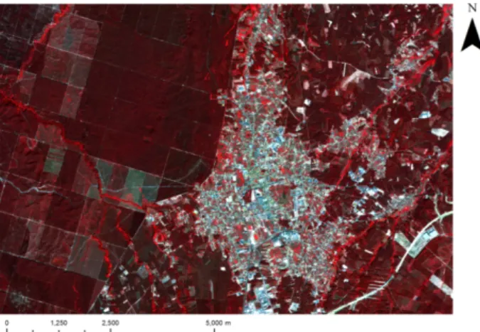
The image data used in this case study was a CARTERRA-Geo image (Jacobsen, 2002) obtained by the IKONOS-2 sensor, with a spatial resolution of 4m in the multispectral mode (XS) (see Figure 1). The image covers an area of 81.5 km2 located near the Portuguese coast, and includes regions with different characteristics, such as built up areas, agricultural fields and forest. The study was performed using the 4 multispectral bands.

Figure 1. False color composition (432) of the multispectral IKONOS image

3.2 Results

3.2.1 Classification: Figure 2 shows the hardened

classification obtained for the multispectral image shown in Figure 1.

Figure 2. Hardened classification of the multispectral image presented in Figure 2, obtained assigning to each pixel the class corresponding to the maximum posterior probability

(4)

3.2.2 Uncertainty and confidence: Figure 3 shows the

spatial distribution the uncertainty obtained with the two uncertainty measures and the classification confidence, and Table 2 the statistical information on the obtained uncertainty and confidence values.

Analysing Figure 3a) and b) and Table 2 it can be seen that the values obtained with the RMD uncertainty measure and the normalized entropy are very similar. The regions with higher values of uncertainty are approximately the same, even though some slightly larger values can be found in some regions with the normalized entropy, confirmed by the fact that the mean value is also slightly higher than the one obtained with the RMD. However, the assessment of the classification confidence produces very different results, as can be seen comparing Figures 3a) and b) with c), where it is clear that the regions presenting less confidence are not the ones that present higher uncertainty according to the normalized entropy and the RMD.

a)

b)

c)

Figure 3. Spatial distribution of the uncertainty obtained with: a) RMD, b) normalized entropy and c) classification

confidence

Figure 4 a), b) and c) show respectively the results obtained for the two uncertainty measures (RMD and normalized entropy) and the levels of confidence. The regions in green correspond to the regions with less uncertainty (low values of RMD and entropy) and high levels of confidence, the yellow regions to the middle levels and the regions in red to the regions with high uncertainty or low confidence, which are expected to have higher levels of classification error and therefore lower values of classification accuracy.

Minimum Maximum Mean Standard Deviation

RMD 0.00 1.00 0.06 0.12

En 0.00 1.00 0.08 0.12

Confidence 1 14 8.26 2.68

Table 2. Statistical information on the pixels uncertainty and confidence values obtained with the RMD, the normalized

entropy (En) and the classification confidence

a)

b)

c)

Figure 4. Regions with high, medium and low uncertainty obtained with a) the RMD uncertainty measure, b) the normalized entropy. Regions with high, medium and low

confidence are shown in c)

(5)

The problematic regions identified with the RMD and the entropy are quite similar. However, the three regions identified with the confidence levels are very different from the ones identified with the two previous uncertainty measures.

3.2.3 Accuracy assessment: The confusion matrixes

constrained to the regions with the three levels of uncertainty obtained with the RMD, normalized entropy and confidence levels were built, and the user’s, producer’s and overall accuracy indices were computed as indicated in section 2.4. As the results obtained with the RMD and the normalized entropy uncertainty measures are almost identical, only the results obtained with the RMD and the classification confidence are shown respectively in Figures 5, 6 and 7.

Figure 5. Overall accuracy of: a) the global image and the regions with low, medium and high uncertainty obtained with the RMD uncertainty measure and b) the global image and the

regions with high, medium and low confidence Figure 5 shows the overall accuracy obtained for the global image and the regions with the three levels of uncertainty obtained with the RMD and the three levels of confidence. The main result that can be observed are that the regions with high uncertainty or low confidence have lower overall accuracy than the regions with lower uncertainty or higher confidence, and that the regions with low and medium uncertainty have higher accuracy that the global image, the same happening with the regions high and medium confidence.

Figure 6. User’s accuracy per class of a) the global image and of the regions with low, medium and high uncertainty computed using the RMD, b) the global image and the regions

with high, medium and low confidence

A similar analysis was done for the user’s and producer’s accuracy per class. Figure 6 shows the user’s accuracy obtained for the several classes for the global image and the regions with the different levels of uncertainty and confidence and Figure 7 the corresponding results obtained for the producer’s accuracy.

Figure 6 shows that the trends observed for the overall accuracy are also observed for the user’s accuracy for the regions with different levels of uncertainty and confidence, with a few exceptions. For the regions defined with the RMD uncertainty measure the user’s accuracy of Forest Areas obtained for the global image and all the regions with different levels of uncertainty are all very similar, with values of, respectively, 89%, 90%, 92% and 84% (Figure 6a). For the class Barren Areas, the regions with low and medium uncertainty have equal values of user’s accuracy (70%), which is much higher than the values obtained for the regions with high uncertainty (42%). For the regions obtained considering the levels of confidence only one exception is observed, for the class Herbaceous Vegetation, but in this case the ordering of the accuracy values is completely inverted in relation to the expected results, with the accuracy increasing with the decrease of confidence. This aspect will be further analyzed in section 3.3.

The results obtained for the producer’s accuracy (Figure 7) are similar to the ones obtained for the user’s accuracy for the class Urban Areas, Forest Areas and Baren Areas. However, large differences can be observed for the classes Herbaceous Vegetation and Shrub Lands, both for the uncertainty and confidence regions. All pixels in the reference database classified as Herbaceous Vegetation were correctly classified in the regions of medium and high uncertainty, resulting in a producer’s accuracy of 100%. On the other hand, the regions with low uncertainty only showed to have a producer’s accuracy of 49%. On the other hand, for the regions with different levels of confidence the accuracy increased with the decrease of confidence (as observed for the user’s accuracy). The same behavior was observed for the producer’s accuracy of class Shrub Lands regarding the different levels of confidence.

Figure 7. Producer’s accuracy per class of a) the global image and of the regions with low, medium and high uncertainty computed using the RMD, b) the global image and the regions

with high, medium and low confidence.

84 89 91 77 0 20 40 60 80 100 Global image Low uncertainty Medium uncertainty High uncertainty Percen ta ge a) 79 88 82 70 0 20 40 60 80 100 Global image High confidence Medium confidence Low confidence Percen ta ge b) 78 60 69 94 55 89 49 93 ₈₉ 78 69 100 42 99 62 55 100 50 90 43 0 10 20 30 40 50 60 70 80 90 100

Urban Areas (UA) Herbaceous

Vegetation (HV)Shrub Lands (SL) Forest Areas (FA) Barren Areas (BA)

Percen ta ge a) Global image Low uncertainty Medium uncertainty High uncertainty 83 46 57 95 56 93 15 38 99 75 88 44 67 94 68 65 71 75 76 44 0 20 40 60 80 100

Urban Areas (UA) Herbaceous

Vegetation (HV)Shrub Lands (SL) Forest Areas (FA) Barren Areas (BA)

Percen ta ge b) Global image High confidence Medium confidence Low confidence

(6)

Figure 8 shows the percentage occupied by each class in the global image and in each of the uncertainty/confidence regions when using the approach described in section 2.3.

Figure 8. Percentage of area assigned to each class in the global image and in the regions with low, medium and high

uncertainty and confidence

It can be seen that the distribution of the classes by the three levels of uncertainty and confidence is in some cases very different from the classes proportion in the global image. For example, most regions that were assigned to medium uncertainty were Forest Areas (90%), which are in most cases well classified (see Figures 6 and 7). Therefore, as the area of the classes occupied in the region under analysis is used to compute the accuracy indices (see section 2.4), this influenced the overall accuracy obtained for this region, resulting in higher values of overall accuracy (91%) when compared to the region with lower uncertainty, that includes mainly Shrub Land (38% of Shrub Land and 34% of Forest Areas).

3.3 Analysis of the regions with different levels of uncertainty and confidence

The analysis of the accuracy of regions with different levels of uncertainty and confidence shows that in general higher levels of uncertainty and lower levels of confidence correspond to lower levels of accuracy. This would enable the identification of regions which are more likely to have classification problems. However, it can be observed in Figure 4 that the regions that may be identified as more problematic using uncertainty and confidence are very different. Moreover, with a fast initial look they even seem to be disjoint. Therefore, a closer analysis per class and levels of uncertainty and confidence needs to be made.

An analysis of the meaning of the uncertainty information shows that both uncertainty measures are obtained using the posterior probabilities computed with equation (2), which express the possibility of existing more than one class candidate to assign to the pixel. This means that lower posterior probabilities are obtained if more candidate classes exist (with similar probabilities) and a posterior probability of one is always obtained if only one candidate class exists, even if the probability obtained with equation (1) is very low. On the other hand, the classification confidence is computed with the values obtained with equation (1) and expresses the proximity of the pixel spectral response to the mean of the probability density function. Therefore, even if no other candidate classes exist, when the pixel spectral response belongs to a confidence interval with a high confidence value (e.g. 0.99) it will always have a low confidence level. Therefore, the uncertainty measures and the classification confidence express different aspects of the classification reliability and have different meanings. The uncertainty expresses the difficulty in choosing one class to assign to the

pixel (high uncertainty values mean that there is difficulty in choosing one class) and the confidence expresses the proximity of the pixel spectral response to the characteristics of the training set of the class to which the pixel was assigned, independently of existing other candidate classes or not. To understand how this influences the distribution of uncertainty and confidence as well as the levels of accuracy obtained in this case study, in this article a more detailed analysis is done by class only for two classes, due to the limitations in space. One of the analysed classes is the class Urban Areas, that shows a decrease in accuracy with a decrease in confidence and increase in uncertainty. The other class analysed is Herbaceous Vegetation, which shows an increase in User’s Accuracy with a decrease in confidence and an increase of the producer’s accuracy both with an increase in uncertainty and a decrease in confidence.

Figure 9 shows the area (in km2_{) of the pixels classified as} Urban that belong to the several combinations of uncertainty and confidence levels and Table 3 shows the distribution of the areas for each confidence level by the three levels of uncertainty. The results show that most regions classified as Urban were classified with low uncertainty (Figure 9 and Figure 8), and from these, most of them have high and medium confidence. That is, most Urban Areas do not have a credible class alternative (have low uncertainty) and have spectral responses close to the class mean (high confidence level). Therefore, as long as the chosen nomenclature has good class separability and there are no classes present in the terrain missing from the nomenclature, it could be expected that higher levels of accuracy would be obtained for these regions. This agrees with what was observed, as the user’s accuracy of the regions with low uncertainty is high (90%). Moreover, the regions with high and medium confidence are almost entirely included in the region with low uncertainty (Table 3), corresponding to subsets of this region with higher accuracy, which corresponds to the obtained results, as the regions with high confidence have a user’s accuracy of 98% and the regions with medium confidence a user’s accuracy of 92%.

Figure 9. Area in km2_{of the region classified as Urban} belonging simultaneously to the indicated levels of uncertainty

and confidence 9 20 2 4 6 10 12 2 2 1 3 1 2 5 22 38 6 21 6 26 46 64 34 90 69 87 61 27 3 6 1 2 0 1 11 0 10 20 30 40 50 60 70 80 90 100

Global image Low

uncertainty uncertaintyMedium uncertaintyHigh ConfidenceHigh ConfidenceMedium ConfidenceLow

Percen

ta

ge Urban Areas (UA)_{Herbaceous Vegetation (HV)}

Shrub Lands (SL) Forest Areas (FA) Barren Areas (BA)

(7)

Low uncertainty (UAc:90%) Medium uncertainty (UAc:72%) High uncertainty (UAc:62%) Region Total High Confidence (UAc: 98%) 94 % 2 % 4% 100% Medium Confidence (UAc: 92%) 85 % 5 % 10% 100% Low Confidence (UAc: 64%) 54 % 13 % 33% 100%

Table 3. Percentage of the pixels classified as Urban Areas with the three levels of confidence that are included in the

three levels of uncertainty. UAc represents the User’s accuracy of each region

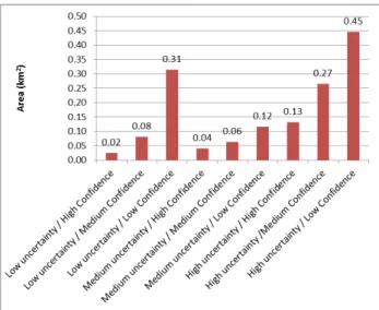
On the other hand, from the regions classified with low confidence, 33% also have high uncertainty. Even though 55% of these regions also have low uncertainty, the user’s accuracy decreased to 64%. A closer analysis of what occurs in the pixels with low confidence and high uncertainty shows that they correspond mainly to pixels difficult to classify and that in many cases are regions of Barren Areas, or in some case Shrubs, which were wrongly classified as Urban Areas. Regarding the class Herbaceous Vegetation, Figure 10 shows the area (in km2_{) of the pixels classified as Herbaceous} Vegetation that belong to the several combinations of uncertainty and confidence levels and Table 4 shows the percentage of pixels classified with low, medium and high levels of confidence that belong to the several levels of uncertainty. The results show that most pixels were classified with high uncertainty, which means that there is at least another candidate class. From these, most of the pixels were also classified with low confidence (0.45 km2_).

Figure 10. Area in km2 of the region classified as Herbaceous Vegetation belonging simultaneously to the indicated levels of

uncertainty and confidence

The results (Table 4) show that most of the pixels classified with high confidence are classified with high uncertainty (67%), which is a region where a user’s accuracy of only 50% was obtained. This explains why the user’s accuracy of the regions with high confidence is so low (only 58%). Moreover, the lower the confidence the higher the percentage of inclusion in the regions with low uncertainty (which has a user’s accuracy of 84% for this class) and the lower the inclusion in the regions with high uncertainty. If the uncertainty is considered as a better indicator of accuracy than confidence, it would be expected that a decrease of the percentage of inclusion in the regions with lower uncertainty would correspond to a decrease in accuracy and an increase in the percentage of inclusion in the regions with high uncertainty would correspond to a decrease of accuracy, which is exactly what is observed. Similar analyses can be made for the other classes, which are not shown here due to space limitations. Low uncertainty (UAc:84%) Medium uncertainty (UAc:78%) High uncertainty (UAc:50%) Region Total High Confidence (UAc: 58%) 12 % 21 % 67% 100% Medium Confidence (UAc: 65%) 20 % 15 % 65% 100% Low Confidence (UAc: 78%) 36 % 13 % 51% 100%

Table 4. Percentage of the pixels classified as Herbaceous Vegetation with the three levels of confidence that are included in the three levels of uncertainty. UAc represents the

User’s accuracy of each region

4. CONCLUSIONS

A methodology was applied in this article to test if the classification uncertainty and/or confidence may be used to identify regions with less accuracy, spatializing therefore the classification accuracy, and providing also a tool to identify regions where the classification may be less reliable, prior to the assessment of classification accuracy. The proposed methodology uses the classification uncertainty computed with the information provided by soft classifiers. In this study a soft Bayesian classifier was used.

As the uncertainty provides information of the classifiers difficulty in assigning only one class to each pixel, as it is more likely to have misclassifications in the regions with higher values of uncertainty, it may provide information about the classification accuracy. This allows the prior identification of regions where different levels of accuracy are expected, allowing the creation of geographically constrained confusion matrixes, which provide information on the spatial distribution of the classification accuracy. Two uncertainty measures were used in this study, namely the RMD and the normalized entropy. Even though these uncertainty measures evaluate different aspects of the classification uncertainty, the obtained results are very similar. This shows that the use of either of these measures does not influence the obtained results. The

(8)

same approach was applied using the information of classification confidence instead of uncertainty, to assess if both indicators (uncertainty and confidence) are good indicators of classification accuracy.

For the identification of the regions with different levels of uncertainty/confidence for the creation of the spatially constrained confusion matrixes, different approaches may be used. This may depend on the characteristics of the spatial distribution of uncertainty and also on the purpose of the application. A simple aggregation of pixels by level of uncertainty was used in this article. However, this approach may generate: 1) regions with little continuity, which may not enable an easy identification of individual meaningful regions, and 2) an uneven distribution of the classes by the different levels of uncertainty/confidence, as can be clearly seen in Figure 8. As the aim in this article was to compare the values of uncertainty/confidence with the classification accuracy, only three levels where considered for the creation of the spatially constrained confusion matrixes. However, the application of such a methodology to identify the problematic regions of each class to identify deficiencies in the used nomenclature regarding the terrain characteristics, or instead of the assessment of the classification accuracy, a different approach needs to be developed, so that the different characteristics of the probability density function of each class is taken into consideration, as well as the separability between classes.

The presented study showed that there is correlation between accuracy, uncertainty and confidence. However, the correlation with uncertainty appears to be a better indicator of classification accuracy than confidence, as the results suggest that the correlation between confidence and accuracy occurs mainly when there is also correlation between confidence and uncertainty. However, the joint use of uncertainty and confidence may allow the creation of an indicator even more reliable than only the classification uncertainty.

The proposed methodology showed therefore to be a promising approach to identify regions with different levels of accuracy of a hardened version of a classification performed with soft classifiers. This information may be quite useful, for example, for reporting the limitations of a land cover map, to identify regions with different characteristics within the same class, for improving classification through the redefinition of the training samples or to be used as an indicator of the classification reliability when an immediate assessment of a land use/land cover map is needed, and no reference data exists to perform a traditional accuracy assessment.

ACKNOWLEDGEMENTS

This research was supported in part by the Portuguese Foundation for Science and Technology (FCT) under project grant UID/MULTI/ 00308/2013.

REFERENCES

Card, D.H., 1982. Using known map category marginal frequencies to improve estimates of thematic map accuracy. Photogrammetric Engineering and Remote Sensing, 48 (3), pp. 431-439.

Congalton, R. G., K. Green, 1999. Assessing the Accuracy of Remotely Sensed Data: Principles and Practices. Lewis Publishers, Boca Raton, FL.

Fonte, C. C., Apolinário, J., Gonçalves, L.M.S., 2013. Assessing the Spatial Variability of Classification Accuracy Using Uncertainty Information. In: 16th AGILE Conference on Geographic Information Science, Leuven, Belgium, May 2013.

Fonte, C. C., Gonçalves, L.M.S., 2011. Assessing the Spatial Variability of the Accuracy of Multispectral Images Classification Using the Uncertainty Information Provided by Soft Classifiers. In: Proceedings of the 7th International Symposium on Spatial Data Quality, Coimbra, Portugal, October 2011.

Foody, G.M., Campbell, N.A., Trodd, N.M., Wood, T.F., 1992. Derivation and applications of probabilistic measures of class membership from maximum likelihood classification. Photogrammetric Engineering and Remote Sensing, 58, pp. 1335-1341.

Gonçalves, L. M., C. C. Fonte, E. Júlio, M. Caetano, 2012. The application of uncertainty measures in the training and evaluation of supervised classifiers. International Journal of Remote Sensing, 33(9), pp. 2851-2867.

Ibrahim, M.A., M.K. Arora and S.K. Ghosh., 2005. Estimating and accommodating uncertainty through the soft classification of remote sensing data. International Journal of Remote Sensing, 26(14), pp. 2995-3007.

Jenks, G. F., 1967. The Data Model Concept in Statistical Mapping. International Yearbook of Cartography 7, pp: 186– 190.

Maselli, F., Conese, C. and Petkov, L., 1994. Use of probability entropy for the estimation and graphical representation of the accuracy of maximum likelihood classifications. ISPRS Journal of Photogrammetry and Remote Sensing, 49 (2), pp. 13-20.

Shi, W. Z., Ehlers, M., Tempfli, K., 1999. Analytical modelling of positional and thematic uncertainties in the integration of remote sensing and geographical information systems. Transactions in GIS, 3 (2), pp. 119-136.