doi: 10.1590/0101-7438.2018.038.01.0153
APPLYING THE TODIM FUZZY METHOD TO THE VALUATION OF BRAZILIAN BANKS
Antonio Marcos Duarte J´unior
Received August 5, 2017 / Accepted March 8, 2018
ABSTRACT.We propose the use of multicriteria decision analysis for the valuation of Brazilian banks. In order to model uncertainties, we combine the use of multicriteria decision analysis with fuzzy mathematics. We specifically modify the methodTomada de Decis ˜ao Interativa Multicrit´erio(TODIM) to incorporate fuzzy numbers, resulting in a methodology we call TODIM Fuzzy. A six-year data set of audited financial statements is considered to illustrate the use of the methodology when analyzing the six largest (net worth) banks operating in Brazil. Several sensitivity analyses are conducted to illustrate how small changes in the inputs can alter the results obtained with the original TODIM and the TODIM Fuzzy. The numerical illustrations have displayed consistent and robust results when the scores of the six banks are computed and the institutions are compared among themselves.
Keywords: fuzzy mathematics, multicriteria decision making, valuation.
1 INTRODUCTION
The valuation of companies can be defined as the process of comparing and ordering their ex-pected performance using to that end financial statements, financial markets data, economic sec-tor analyses and projected economic scenarios (Clayman et al., 2016). The financial analysts most often select different economic, accounting and financial indicators, commonly referred to as “multiples”, to understand the relative prospects of companies based on financial concepts such as value, liquidity, return, risks and costs (Damodaran, 2012; Stowe et al., 2014).
The Multicriteria Decision Analysis (MCDA) allows a decision maker to obtain compromise so-lutions when facing the problem of selecting among several alternatives using to the end a set of criteria (Belton & Stewart, 2002; Figueira et al., 2005; Ishizaka & Nemery, 2013; Wallenius et al., 2008). Examples of MCDA applied to accounting and finance are quite diversified in the international literature (Gu et al., 2017, Hallerbach & Spronk, 2002; Steuer & Na, 2003; Xidonas et al., 2011; Xidonas et al., 2012; Zavadskas & Turskis, 2011, Zouponidis et al., 2015, among
others). However, the analysis of financial institutions remains restricted to credit rating analy-sis, as illustrated by Doumpos & Zouponidis (2011), with no specific article on their financial valuation.
The use of several criteria to compare a set of alternatives is the typical problem considered in MCDA. In other words, once the financial analyst has selected the set of multiples (i.e., crite-ria) he intends to use to compare financial institutions, the MCDA turns out to be an interesting framework to model de valuation problem, facilitating the comparison of companies (i.e., alter-natives) to rank them form the most to the least promising in terms of expected performance.
The multiples used in valuation carry uncertainties in their values, since they result from finan-cial projections obtained by the analysts. One interesting possibility to model uncertainties in the valuation problem is to rely on fuzzy mathematics (Bellman & Zadeh, 1970; Kaufmann & Gupta, 1985; Klir & Yuan, 1995; Zadeh, 1965). Therefore, it is important to modify MCDA methodolo-gies to incorporate fuzziness before they are applied to the valuation problem (Kahraman, 2008; Pedrycz et al., 2011; Zimmermann; 1991).
Our main objective in this work is to propose and illustrate the use of MCDA to the valuation of companies. We propose a methodology that allows the decision maker to compute scores/grades for the companies of interest, so that their projected future performances can be compared. It is opportune to mention that there is no literature published on the use of MCDA for the valuation of companies. Since valuation is a quite broad theme, we concentrate in a specific economic sector for illustrative purposes: the Brazilian banking sector. We consider performing the valuation of the six largest banks (net worth) operating in Brazil.
Our secondary objective is to model uncertainty in the valuation problem of Brazilian companies. In line with the abovementioned literature, we propose modifying the methodTomada de Decis˜ao Interativa Multicrit´erio(TODIM; Gomes & Lima, 1991, 1992) to incorporate fuzzy numbers. A fuzzy version for the TODIM method is detailed, which we refer to simply as TODIM Fuzzy from now on. Several sensitivity analyses are performed and commented to understand how the scores obtained are altered as various levels of uncertainty (symmetric and asymmetric) are incorporated in the multiples. Our focus (with the sensitivity analyses) is to compare how the results obtained with the original TODIM and the TODIM Fuzzy differ for different levels of uncertainty in the multiples and their relative importance.
2 VALUATION USING MCDA AND FUZZY MATHEMATICS
The general framework for the valuation problem we propose, with MCDA and fuzzy mathemat-ics, builds on the steps described in three books on the subject (Clayman et al., 2016; Damodaran, 2012; Stowe et al., 2014).
The first step necessary to perform a valuation requires identifying the set of multiples to be used in the analysis. The set of multiples is very dependent on the economic sector of interest (Stowe et al., 2014): for example, the multiples used to analyze banks differ from those used to analyze transportation companies. In this work, as already mentioned, we concentrate on the Brazilian banking sector for the sake of illustration. We select multiples for the numerical examples from technical reports issued by the research areas of three investment banks, as detailed later.
The second step requires establishing the relative importance of the previously selected multi-ples. In other words, it is necessary that the financial analyst completely specifies for each pair of criteria which one is the most important (or, that they are equally important) when analyzing the chosen companies. This can be achieved by the specification of the pairwise comparative matrix, according to Gomes & Lima (1991, 1992). It is also important to mention that the relative im-portance of criteria most probably will differ from one financial analyst to the other, this being a personal preference decision according to Damodaran (2012).
The third step involves selecting the companies that are to be compared within the economic sector of interest. Our interest when using a MCDA method is to establish a comparison between each pair of companies, indicating which should be considered dominant over the other in terms of expected performance. The banks used in the numerical examples are the largest in Brazil when compared by their net worth.
The fourth step requires the selection of a MCDA method. There is a quite large number of possibilities, we must say. For the sake of illustration, we have chosen TODIM. It is theoretically sound and has been widely used by academics and practitioners (Dehghani et al., 2017; Gomes et al., 2010; Gomes & Rangel, 2009; Jiang et al., 2017; Kazancoglu & Burmaoglu, 2013; Krohling & Souza, 2012; Lee & Shih, 2016; Lisboa & Duarte, 2013; Liu & Teng, 2015; Lourenzutti & Krohling, 2013; Lourenzutti & Krohling, 2015; Qin et al., 2017; Qin et al., 2017; Ren & Xu, 2016; Wang et al., 2017; & Xu, 2014; Zhang et al., 2017; among others). In addition, TODIM can be easily implemented from the computational point of view: our numerical examples were obtained using the software MATLAB. Another interesting point is that TODIM provides, at the end of its execution, scores for the alternatives in the normalized interval [0,1], facilitating post-execution analyses.
In the sixth (and last) step, the actual application of the fuzzy MCDA to the data takes place. The final output is a set of scores, one for each company analyzed. These scores are to be subjected to sensitivity analyses to understand how changes in the input can alter them. Finally, the final ordering according to the obtained expected performances can be established.
In the remaining of this section, we customize the framework above for the numerical examples presented later.
2.1 Multiples
The first step of a valuation process requires specifying the multiples for the analysis of com-panies in a specific economic sector. As already mentioned, there can be many multiples when valuing companies. MCDA is suited for the analysis of companies with many criteria and, conse-quently, can appropriately handle any number of multiples. It makes no sense, however, to use a large number of multiples in an academic work, given conciseness and space limitation, besides the fact that we need to provide numerical examples for illustrative purposes only. Therefore, we chose a reasonable number (i.e., nine multiples) for the numerical examples, following a two-step process.
The first step established the main areas where we should have multiples present. We have chosen six main areas, in line with the technical report Basel Committee on Banking Supervision (2011): solvency/risk, profitability/return, credit exposures, liquidity, operational costs and asset-liability structure. In other to select the multiples, in the second step, we perused technical reports pro-duced in a five-year period (2009-2014) by the research areas of three very active investment banks (BTF Pactual, Credit Suisse and Goldman Sachs), taking notes of the multiples adopted by their professionals when analyzing the Brazilian banking sector. We were finally able to iden-tify nine multiples as the most often adopted: one for risk/solvency, two for return, two for credit exposures, two for liquidity, one for operational costs and one for asset-liability structure. These multiples are explained next.
The first multiple is the Basel Index (BI; Basel Committee on Banking Supervision, 1988), re-lated to risk/solvency. The BI determines the minimum regulatory capital required by the Banco Central do Brasil for all banks operating in the country. It has been in effect globally since 1988 and, in Brazil, since 1994, following the Resoluc¸˜ao CMN 2099/94. The computation of the BI evolved substantially after 1994, especially after the Basel Accord II and the Basel Accord III (Basel Committee on Banking Supervision, 2005, 2011), but its interpretation for financial ana-lysts remains the same: the larger the BI, the larger the solvency probability of the bank (Laeven & Levine, 2009).
The third multiple is the Return on Asset (ROA), also a profitability indicator, as the ROE. The ROA measures the bank capacity to generate net income for each monetary unit of its total asset. For example, if the ROA is computed at 2%, we can interpret that for each R$100 of assets, the bank generates a profit of R$2. Once more, the higher the ROA, the better should the expected performance of a bank be considered.
The fourth multiple is the Regulatory Provisioning (RP) amount required by the Banco Central do Brasil from all banks operating in local financial market. RP measures the percentage of the total credit exposure expected to become “default” according to the rating system originally described in the Resoluc¸˜ao CMN 2682/99. For example, if the RP of a bank is estimated at 4%, for each R$100 of credit exposure, R$4 are expected not to be repaid. In the case of this indicator, the larger its value, the larger the expected credit losses and, consequently, the worse the expected performance of the bank.
The fifth multiple is an estimate of the amount of credit already expired for at least thirty days (CE30), computed as a percentage of the total credit exposure. For example, if the CE30 of a bank is calculated at 1%, we can say that for every R$100 of credit exposure, R$1 has expired but has not been repaid by the counterparties/borrowers for at least thirty days. The CE30 is related to the RP, but financial analysts think this to be such an important information in the case of banks, that we decided to compute it separately. Again, as in the case of RP, the larger the value of CE30, the worse should be considered the bank expected performance.
The sixth multiple is the Liquidity Ratio (LR), computed as the ratio of the summation of the current assets and investments, divided by the summation of current liabilities and long-term liabilities. This multiple can be used as an indicator for the long-term liquidity of the financial institution (Damodaran, 2012). The large this multiple, the better should be the expected perfor-mance of the financial institution in the long term.
The seventh multiple is the Current Ratio (CR), also a liquidity indicator, computed as the ratio of the current assets by the current liabilities, differing from the LR because it is concentrated in the short term. In other words, the CR can be used to better understand the short-term liquidity necessities of a financial institution, while the LR the long-term necessities. The CR must be interpreted the same way as the LR: the larger the CR, the less probable that liquidity problems affect the financial institution and, consequently, the better should be its expected performance.
The eight multiple is a measure of Operational Cost (OC), computed as the ratio between the summation of all taxes, administrative and personnel expenses, and the summation of revenues services and brokerage fees. Although there are several possible indicators for operational costs (Clayman et al., 2016), this is a specific measure used by all banking analysts, this being the reason why it was chosen. Since this multiple is a cost, the larger its value, the worse the expected performance of the financial institution.
multiple Ob, the worse should be the performance of the financial institution given the higher probability that it may experience difficulties handling its liabilities in the future.
TODIM requires all multiples to be “benefits” (the larger its value, the better) or “costs” (the smaller its value, the better), according to Gomes & Lima (1991, 1992). Since four of the multi-ples just described are “costs”, we chose to transform them to become “benefits” by taking their inverse values.
We also take this opportunity to mention that incorporating or removing multiples when using our proposal is a straightforward task. In other words, the financial analyst can easily experiment with different sets of multiples when analyzing companies with the use of the methodology proposed in this work.
2.2 Banks
We have chosen the Brazilian banks for the numerical illustrations according to their net worth at the end of 2014: all banks with a net worth above US$5 billion were selected. Accord-ing to their audited financial statements, Ita´u (US$ 38.8 billion), Bradesco (US$ 30.7 billion), Banco do Brasil (US$ 26.6 billion), Santander (US$ 21.1 billion), Caixa Econˆomica Federal (US$ 9.8 billion) and BTG Pactual (US$ 5.5 billion) all qualified. Three comments are important at this point:
i. We have disregarded BNDES (US$ 11.6 billion) given its special characteristics, as a not-for-profit national development bank.
ii. We have not disregarded BTG Pactual, although it can be considered closer to invest-ment banks than commercial banks, as it is the case of the other five selected institutions. We mention that we ran two batches of numerical examples: one with BTG Pactual, one without it. We preferred to report the results in this work with all six banks together.
iii. From now on, we will refer to the banks simply as B1, . . . , B6, because their names are unimportant to the conclusions of this work. Obviously, any financial analyst that follows closely the Brazilian-banking sector will easily identify the banks from the data displayed next.
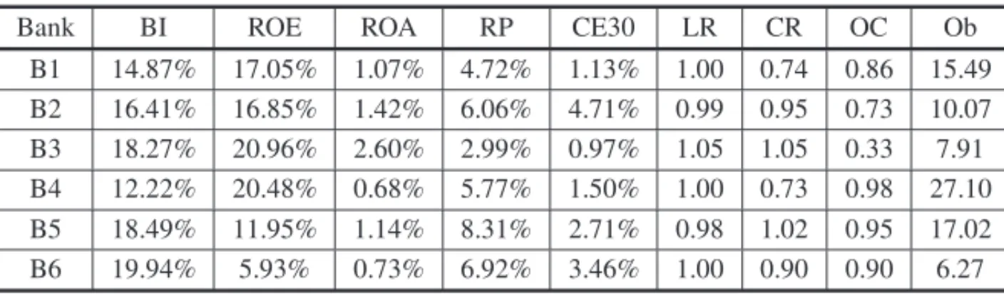
We selected a six-year period (2009-2014) of audited financial statements to compute the nine multiples for each bank. Table 1 summarizes the mean obtained for the multiples of the six banks considered.
Naturally, when financial analysts compare banks using multiples, they do so after projecting theses values in the future. This observation leads us to the problem of modeling uncertainty in the valuation process. As already said, we suggest in this work the use of fuzzy mathematics to capture uncertainty into valuation.
Table 1– Data for Six Banks (2009-2014).
Bank BI ROE ROA RP CE30 LR CR OC Ob
B1 14.87% 17.05% 1.07% 4.72% 1.13% 1.00 0.74 0.86 15.49
B2 16.41% 16.85% 1.42% 6.06% 4.71% 0.99 0.95 0.73 10.07
B3 18.27% 20.96% 2.60% 2.99% 0.97% 1.05 1.05 0.33 7.91
B4 12.22% 20.48% 0.68% 5.77% 1.50% 1.00 0.73 0.98 27.10
B5 18.49% 11.95% 1.14% 8.31% 2.71% 0.98 1.02 0.95 17.02
B6 19.94% 5.93% 0.73% 6.92% 3.46% 1.00 0.90 0.90 6.27
membership functions used in the numerical examples. For example, if we consider bank B5 and the multiple BI, the membership function of this fuzzy number will attain its maximum value (equal to one) at 18.49%, with the decay (of the membership function) above and below varying according to the level of uncertainty assumed by the financial analyst. We shall illustrate this in detail later.
2.3 Scores
TODIM Fuzzy offers, at the end of its execution, a set of scores for the banks considered for analysis. These scores are to be thoroughly analyzed with the use of sensitivity analyses. The largest scores obtained (close do one) are related to the most interesting banks in terms of future performance, which should be deemed “preferred” by any financial analyst.
3 TODIM FUZZY
We detail in this section the TODIM Fuzzy version used in the numerical problems presented later in this work. This version builds on the original TODIM (Gomes & Lima, 1991, 1992) by incorporating fuzzy numbers. Other versions of the TODIM Fuzzy have already been applied to different areas of engineering, logistics and supply chain management (Li et al., 2015; Louren-zutti & Krohling, 2013; Ramooshjan et al., 2015; Tosun & Akyuz, 2014, among others), with no examples so far in the finance and accounting areas.
It is possible to adapt the original TODIM to incorporate fuzzy mathematics in different ways. In the presentation below, we use triangular numbers, although other fuzzy numbers (trapezoidal, bell-shaped etc.) can be used, as illustrated in Li et al. (2015). In addition, it is possible to incorporate concepts extracted from the Prospect Theory (Kahneman & Tversky, 1979) as in Ramooshjan et al. (2015) and Tosun & Akyuz (2014), although we choose to use a linear utility function, which greatly simplifies the presentation and computations. Finally, the defuzzification process can be quite varied (Leekwijck & Kerre, 1999), but we preferred to utilize it as detailed below (center of gravity, with squared distances), which neatly simplifies in the final formula.
specify precisely the relative importance of multiples and, thus, it becomes important to incor-porate fuzziness in the weight vector, as detailed below. In other words, uncertainties are not restricted anymore only to the data matrix (i.e., multiples), but can be incorporared also in the relative importance of all criteria, extending the modelling of uncertainties in the TODIM Fuzzy.
We denote the fuzzy data matrix as
⎛ ⎜ ⎜ ⎜ ⎜ ⎜ ⎜ ⎜ ⎜ ⎝
d11(1);d11(2);d11(3) d12(1);d12(2);d12(3) · · · d1(1n);d1(2n);d1(3n)
d21(1);d21(2);d21(3) d22(1);d22(2);d22(3) · · · d2(1n);d2(2n);d2(3n)
.. .
dm(11);dm(21);dm(31)
.. .
dm(12);dm(22);dm(32)
. ..
· · ·
.. .
dmn(1);dmn(2);dmn(3) ⎞ ⎟ ⎟ ⎟ ⎟ ⎟ ⎟ ⎟ ⎟ ⎠ (3.1)
for which we assume that 0<di j(1)≤di j(2)≤di j(3),i=1, . . . ,mand j =1, . . . ,n. The membership function for a triangular fuzzy number can be written as
Ŵ
di j(1);d(i j2);di j(3)(y)= ⎧ ⎪ ⎪ ⎪ ⎪ ⎪ ⎪ ⎨ ⎪ ⎪ ⎪ ⎪ ⎪ ⎪ ⎩
y−di j(1) di j(2)−di j(1) d
(1)
i j ≤y<d (2) i j
d(i j3)−y di j(3)−di j(2) d
(2)
i j ≤ y≤d
(3) i j
0 otherwise
∀i =1, . . . ,mand
j =1, . . . ,n. (3.2)
The normalized fuzzy data matrix can be obtained from (3.1), with its generic element given by
ai j(1);ai j(2);ai j(3)
=
⎛
⎝
di j(1)
maxd1(2j), . . . ,dm j(2) ;
di j(2)
maxd1(2j), . . . ,dm j(2) ;
di j(3)
maxd1(2j), . . . ,dm j(2)
⎞
⎠ (3.3)
where it can be verified that 0<ai j(2)≤1 fori=1, . . . ,mand j=1, . . . ,n. The normalized matrix can be written as
⎛ ⎜ ⎜ ⎜ ⎜ ⎜ ⎜ ⎜ ⎜ ⎝
a11(1);a11(2);a(113) a12(1);a12(2);a12(3) · · ·
a1(1n);a1(2n);a1(3n)
a21(1);a21(2);a21(3) a22(1);a22(2);a22(3) · · · a2(1n);a2(2n);a2(3n)
.. .
am(11);am(21);a(m31)
.. .
am(12);am(22);am(32)
. ..
· · ·
.. .
amn(1);amn(2);amn(3) ⎞ ⎟ ⎟ ⎟ ⎟ ⎟ ⎟ ⎟ ⎟ ⎠ (3.4)
with a membership function as
Ŵ
a(i j1);a(i j2);a(i j3)(y)= ⎧ ⎪ ⎪ ⎪ ⎪ ⎪ ⎪ ⎨ ⎪ ⎪ ⎪ ⎪ ⎪ ⎪ ⎩
y−ai j(1) a(i j2)−a(i j1) a
(1)
i j ≤ y<a (2) i j
a(i j3)−y a(i j3)−a(i j2) a
(2)
i j ≤y≤a
(3) i j
0 otherwise
∀i=1, . . . ,m and
We denote the fuzzy weight vector (with the relative importance of thencriteria) as
h1(1);h(12);h1(3);h(21);h2(2);h(23);. . .;hn(1);h(n2);h(n3) (3.6) for which we assume, without loss of generality, that
0<h(j1)≤h(j2)≤h(j3) ∀ j =1, . . . ,n.
The final fuzzy weight vector is
w1(1);w(12);w1(3);w(21);w2(2);w2(3);. . .;wn(1);wn(2);wn(3) (3.7) with its generic element given by
w(j1);w(j2);w(j3)
=
⎛
⎝
h(j1)
maxh(12), . . . ,h(n2)
;
h(j2)
maxh(12), . . . ,h(n2)
;
h(j3)
maxh(12), . . . ,h(n2)
⎞
⎠ (3.8)
which satisfies 0 < w(j2) ≤ 1 for j =1, . . . ,n. The membership function for each element of the final weight vector is written as
Ŵ
w(j1);w(j2);w(j3)(y)= ⎧ ⎪ ⎪ ⎪ ⎪ ⎪ ⎪ ⎨ ⎪ ⎪ ⎪ ⎪ ⎪ ⎪ ⎩
y−w(j1) w(j2)−w(j1) w
(1)
j ≤y< w (2) j
w(j3)−y w(j3)−w(j2) w
(2)
j ≤y≤w
(3) j
0 otherwise
∀ j=1, . . . ,n (3.9)
The relative dominance fuzzy matrix is such that its generic element is obtained from
δil(1);δil(2);δil(3)=
n
j=1
w(j1);w(j2);w(j3)×a(i j1);ai j(2);a(i j3)−al j(1);al j(2);al j(3) (3.10)
fori =1, . . . ,mandl=1, . . . ,m. The fuzzy dominance vector results to be
γi(1);γi(2);γi(3)=
m
l=1
δil(1);δil(2);δil(3) (3.11)
fori = 1, . . . ,m. Again, the membership function for each element of the fuzzy dominance vector is given by
Ŵ
γj(1);γ(j2);γj(3)(y)= ⎧ ⎪ ⎪ ⎪ ⎪ ⎪ ⎪ ⎨ ⎪ ⎪ ⎪ ⎪ ⎪ ⎪ ⎩
y−γj(1) γj(2)−γ(j1) γ
(1)
j ≤y< γ (2) j
γ(j3)−y γj(3)−γ(j2) γ
(2)
j ≤y≤γ
(3) j
0 otherwise
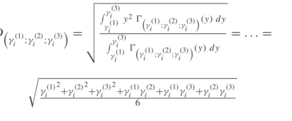
The defuzzification process applied to the fuzzy dominance vector is
D
γi(1);γi(2);γi(3) =
γ
(3)
i
γ(1)
i y2Ŵ
γ(1)
i ;γ
(2)
i ;γ
(3)
i
(y)d y
γ
(3)
i
γ(1)
i Ŵ
γ(1)
i ;γ
(2)
i ;γ
(3)
i
(y)d y
=. . .=
γi(1)2+γi(2)2+γi(3)2+γi(1)γi(2)+γi(1)γi(3)+γi(2)γi(3) 6
(3.13)
fori =1, . . . ,m.
The final ordering can be obtained with the best possibility corresponding to the maximum value (i.e., max{D
(γ1(1);γ1(2);γ1(3));. . .;D(γm(1);γm(2);γm(3))}), and so on until the worst alternative, cor-responding to the minimum value (i.e., min{D
(γ1(1);γ1(2);γ1(3));. . .;D(γm(1);γm(2);γm(3))}).
An interesting point to mention about the version of the TODIM Fuzzy presented above is that it captures precisely the original TODIM if the minimum and maximum value of all triangular fuzzy numbers (multiples and relative importance) are set equal, contrary to what happens with other works, such as Ramooshjan et al. (2015) and Tosun & Akyuz (2014).
4 NUMERICAL RESULTS
As a first numerical illustration, let us consider that the data in Table 1 correspond to the pa-rametersdi j(2)in (3.1). The levels of uncertainty (above and belowdi j(2)) are assumed initially at
±10%, meaning that
di j(1);di j(2);di j(3)=90%×di j(2);di j(2);110%×di j(2) ∀i,j. (4.1)
We assume also in this first numerical example that all the components h(12), . . . ,h(92) of the weight vector (3.6) are equally important, according to Table 2. The levels of uncertainty of the fuzzy weight vector are assumed to be±5%, implying that
h(j1);h(j2);h(j3)=95%×h(j2);h(j2);105%×h(j2) ∀ j (4.2)
Table 2– Original Weight Vector.
BI ROE ROA RP CE30 LR CR OC Ob
1 1 1 1 1 1 1 1 1
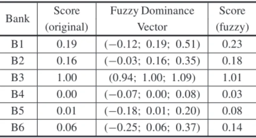
Table 3 summarizes the scores obtained for the original TODIM and the TODIM Fuzzy:
ii. The third column displays the fuzzy dominance vector obtained with the TODIM Fuzzy. These values can be compared to those obtained with the original TODIM to better under-stand how fuzziness alters the scores.
iii. The fourth column displays the scores obtained after applying the defuzzification process to the fuzzy dominance vector, according to (3.13).
We can reach some conclusions from Table 3:
i. If we consider only the fuzzy dominance vector, we can observe a considerable overlap among its fuzzy elements, except for B3, meaning the it has an undisputed superior ex-pected performance.
ii. We can also observe that incorporating uncertainties into the valuation process leads to quite different impacts over the fuzzy scores: the minimum impacts are over B4(0,08+
0,07=0,15)and B3(1,09−0,94=0,15), while the two largest impacts happen over B1(0,51+0,12=0,67)and B6(0,37+0,25=0,62).
iii. We can observe that the orderings obtained with the original TODIM and the TODIM Fuzzy (after defuzzification) were the same. Let us not forget that not only the ordering is important in this problem, but also the scores, which can be used, for instance, to establish “ratings” for the future expected performance of companies, similarly to what was illus-trated in Doumpos & Zouponidis (2011) for the credit analysis of issuers in the corporate bond markets, as well as in Silva et al. (2007) in the case of Brazilian computer compa-nies seeking credit from FINEP. Clearly, if a financial analyst has the possibility to obtain the scores for those companies of interest from a methodology that explicitly considers uncertainties, this methodology should be considered superior from the modelling point of view when compared to alternatives that disregard the uncertainties naturally present in the multiples and the components of the weight vector.
Table 3– Scores and Fuzzy Dominance Vector.
Bank Score Fuzzy Dominance Score
(original) Vector (fuzzy)
B1 0.19 (−0.12;0.19; 0.51) 0.23 B2 0.16 (−0.03;0.16; 0.35) 0.18 B3 1.00 (0.94;1.00;1.09) 1.01 B4 0.00 (−0.07;0.00; 0.08) 0.03 B5 0.01 (−0.18;0.01; 0.20) 0.08 B6 0.06 (−0.25;0.06; 0.37) 0.14
can be achieved with the use of the TODIM Fuzzy, but not with the original TODIM, another unmistakable evidence favoring the former over the later. In other words, the use of TODIM Fuzzy allows the financial analyst to experiment with distinct scenarios, related to various lev-els of uncertainties, symmetric or not, which is a major modelling flexibility (and consequently, advantage) over the use of the original TODIM.
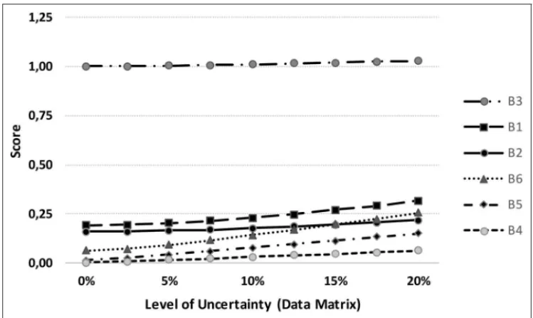
As a first set of sensitivity analysis, we consider experimenting with different levels of uncer-tainty in the fuzzy data matrix (3.1). We can observe from equation (4.1) that the results in Table 3 were obtained with a level of uncertainty equal to±10%. We consider now varying the levels of uncertainty according to nine possibilities: 0%,±2.5%,±5%,±7.5%,±10%,±12.5%,
±15%,±17.5% and±20%. In other words, we set the level of uncertainty at 0% and obtain the defuzzified scores for the six banks, repeating the computations for±2.5% and so on, until we reach the maximum level uncertainty used at±20%. In addition, in this first set of sensitivity analysis we keep the weight vector as used to obtain Table 3 (i.e., the level of uncertainty at
±5%, around the values given in Table 2). Figure 1 depicts the results obtained, where we can observe a smooth tendency for the defuzzified scores to rise as the level of uncertainty increases for all six banks considered, without discontinuities and, also, the maintenance of the ordering displayed at Table 2 with a single exception (B2 and B6, for larger levels of uncertainty).
Figure 1– Sensitivity Analysis of the Fuzzy Data Matrix.
summarized in Figure 2, where we can observe a very smooth rising tendency of the defuzzified scores, with no changes in the orderings displayed in Figure 2.
Figure 2– Sensitivity Analysis of the Fuzzy Weight Vector.
The third sensitivity analysis performed aims at understanding how the relative importance of the multiple BI impacts the scores and the orderings in Table 3. In other words, we increase the importance of this multiple, keeping all others fixed, thus conferring more importance for BI with respect to all other multiples. The results displayed in Table 3 were obtained with the weights in Table 2, whereh(BI2) = 1, with the fuzzy weight component related to BI given by
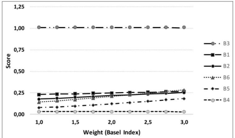
(0.95;1.00;1.05). In this third sensitivity analysis, we varyh(BI2)sequentially for the values 1.00, 1.25, 1.50, 1.75, 2.00, 2.25, 2.50, 2.75 up to 3.00, keeping the corresponding values of all other multiples fixed at 1,00. The level of uncertainty for the components of the fuzzy data matrix is maintained fixed at±10%, while the corresponding level of uncertainty in the components of the fuzzy weight vector is kept at±5%. The results are exhibited in Figure 3, where we observe that with the increase of the relative importance of the multiple BI, the defuzzified scores of banks B2, B6 and B5 tend to increase substantially, given their prudent amount of regulatory capital, this not being the case of B3 and B4, which show a small decrease of their scores.
As a fourth illustration, we consider the comparison of the six banks using only the five multiples related to solvency, return and credit exposures (i.e., BI, ROE, ROA, RP and CE30), three of which are very specific and applied only to the banking sector.
We assume the multiples to be equally important
i.e.,h(BI2)=hROE(2) =hROA(2) =h(RP2)=h(CE302) =1
Figure 3– Sensitivity Analysis for the Weight of the Multiple BI.
Table 4 exhibits the fuzzy dominance vector and the defuzzified scores, which should be com-pared to the values in Table 3. We can observe a much better relative expected performance of B1, B2 and B4, and a worse relative performance in the case of bank B6, all direct consequences of the good quality of the credit exposures of B1, B2 and B4.
Table 4– Results Obtained with Five Multiples (BI, ROE, ROA, RP and CE30).
Bank Fuzzy Dom. Vector Score B1 (0.22; 0.45;0.68) 0.46 B2 (0.10; 0.22;0.35) 0.23 B3 (0.96; 1.00;1.07) 1.01 B4 (0.22; 0.28;0.34) 0.28 B5 (0.00; 0.14;0.28) 0.15 B6 (−0.21;0.00;0.20) 0.08
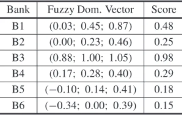
So far, we have considered only symmetric uncertainties in the fuzzy components of (3.1) and (3.6). In this fifth numerical illustration, we exemplify modeling worsening economic conditions and their impact in the banking sector with the use of asymmetrical uncertainties. For example, using only the five multiples of the preceding example (BI, ROE, ROA, RP and CE30), a financial analyst can simulate the effects of an economic recession on the expected performance of the six banks.
exposures of all banks tend to be downgraded, leading to higher requirements for regulatory provisions and solvency capital, reducing profitability, and at the end, increasing multiples such as RP and CE30, while at the same time decreasing the three others, BI, ROE and ROA.
We consider modeling uncertainties in this fifth example as follows:
i. The levels of uncertainty of the multiples BI, ROE and ROA are modeled as−30% and
+10% for the lower and upper limits of the triangular fuzzy numbers, respectively. For example, the bank B1 has as its component for the multiple BI in (3.1) the fuzzy triangular number(70%×14.87%; 14.87%; 110%×14.87%) = (10.41%; 14.87%; 16.36%), with more uncertainty below the level 14.87% than above it, resulting in the asymmetry wanted.
ii. The levels of uncertainty of the multiples RP and CE30 are modeled as−10% and+30% for the lower and upper limits of the triangular fuzzy numbers, respectively. For example, the bank B3 has as it component for the multiple RP in (3.1) the fuzzy triangular num-ber (90%×2.99%; 2.99%; 130%×2.99%) = (2.69%; 2.99%; 3.89%), with more uncertainty above the level 2.99% than below it, resulting in the asymmetry wanted.
iii. The five multiples are kept as equally important in the valuation process
i.e.,h(BI2) =
hROE(2) = h(ROA2) = hRP(2) = h(CE302) = 1
,with a symmetrical level of uncertainty at ±5% in (3.6).
Table 5 resumes all results obtained in the asymmetric case, and should be compared to the value displayed in Table 4, obtained for the symmetric case. We can observe increases in the scores of all banks, except B3. Among the increases, the largest observed was related to banks B6 (from 0,08 to 0,15). No changes were observed in the orderings, despite the scores changes.
Table 5– Results Obtained with Five Multiples and Asymmetric Uncertainties.
Bank Fuzzy Dom. Vector Score B1 (0.03;0.45;0.87) 0.48 B2 (0.00;0.23;0.46) 0.25 B3 (0.88;1.00;1.05) 0.98 B4 (0.17;0.28;0.40) 0.29 B5 (−0.10;0.14; 0.41) 0.18 B6 (−0.34;0.00; 0.39) 0.15
5 CONCLUSION
provided meaningful results when applied to data from the Brazilian banking sector. Several sensitivity analyses were performed to help understand how the results obtained with the origi-nal version of TODIM and the TODIM with fuzziness compared between themselves. Also, we experimented with symmetric and asymmetric fuzzy numbers, illustrating how to incorporate worsening scenarios in the valuation of banks. At this point, it is worth remembering that there are no works with applications of MCDA and fuzzy mathematics to the valuation of Brazilian companies in the academic literature.
Valuation is a quite broad theme in accounting and finance, meaning that it is possible to modify this work in several ways. For example, it is possible to investigate the performance of the pro-posal when applied to different economic sectors (i.e., in addition to the banking sector). Since each economic sector has its own group of multiples, the analysis of different economic sectors will require changing the set of multiples. In this work, we showed how the results were altered when using nine multiples, or a smaller set, with only five multiples. We also illustrated how to remove and incorporate new multiples into the valuation process.
We also experimented with the use of symmetric and asymmetric uncertainties, in order to under-stand how this change can impact the final scores. The particular numerical illustration presented considered modelling a scenario where the economic outlook for the banking sector was bearish, meaning that difficult times should have been expected ahead. Again, the methodology proposed performed quite well, providing the decision maker with detailed information for a solid analysis.
From the MCDA point of view, it is possible to modify this work by the use of different method-ologies. Several MCDA methods can be used by academics and practitioners to the valuation problem (for example, AHP, TOPSIS etc.), we have chosen to apply the TODIM method in this work because it has been widely and successfully applied to the solution of a broad range of engineering and general management problems. One possible extension of this work is to apply other fuzzy MCDA methods to understand how their outputs compare to the results presented in the preceding section. We take this opportunity to mention that we did a limited experiment with a fuzzy version of TOPSIS, with basically the same final results (i.e., orderings were the same) from those displayed in this work for TODIM.
Finally, it is also possible to experiment with other fuzzy numbers (trapezoidal, bell-shaped etc.). We also performed a limited number of numerical experiments with trapezoidal fuzzy numbers and TODIM, with no important changes in the final results (i.e., the same orderings were obtained as those displayed for triangular numbers).
REFERENCES
[1] BASEL COMMITTEE ON BANKING SUPERVISION. 1988. International Convergence of Capital Measurement and Capital Standards.Basel: Basel Committee on Banking Supervision.
[3] BASELCOMMITTEE ONBANKINGSUPERVISION. 2011.A Global Regulatory Framework for More Resilient Banks and Banking Systems.Basel: Basel Committee on Banking Supervision.
[4] BELLMANBE & ZADEHLA. 1970. Decision-making in a Fuzzy Environment.Management Sci-ence,17(1): 141–164.
[5] BELTONV & STEWARTTJ. 2002.Multiple Criteria Decision Analysis: An Integrated Approach. New York: Springer.
[6] CLAYMANMR, FRIDSONMS & TROUGHTONGH.Corporate Finance: A Practical Approach. New York: Wiley.
[7] DAMODARANA. 2012.Investment Valuation. New York: Wiley.
[8] DOUMPOSM & ZOPOUNIDISC. 2011. A Multicriteria Outranking Modeling Approach for Credit Rating.Decision Sciences,42(1): 721–742.
[9] DEHGHANIH, SIAMIA & HAGHIP. 2017. A New Model for Mining Method Selection Based on Grey and TODIM Methods.Journal of Mining and Environment,8(1): 49–60.
[10] FIGUEIRAJ, GRECOS & EHGOTTM (Eds.). 2005.Multiple Criteria Decision Analysis: State of Art Surveys. Berlin: Springer.
[11] GOMESCFS, GOMESLFAM & MARANHAO˜ FJC. 2010. Decision Analysis for the Exploration of Gas Reserves: Merging TODIM and THOR.Pesquisa Operacional,30(1): 601–617.
[12] GOMESLFAM & LIMAMMPP. 1991. TODIM: Basics and Application to Multicriteria Ranking of Projects with Environmental Impacts.Foundations of Computing and Decision Sciences,16(1): 113–127.
[13] GOMES LFAM & LIMA MMPP. 1992. From Modeling Individual Preferences to Multicriteria Ranking of Discrete Alternatives: Look at the Prospect Theory and the Additive Differences Model. Foundations of Computing and Decision Science,1791: 171–184.
[14] GOMESLFAM & RANGELLAD. 2009. An Application of the TODIM Method to the Multicrite-ria Rental Evaluation of Residential Properties.European Journal of Operational Research,193(1): 204–211.
[15] GUW, BASUM, CHAOZ & WEIL. 2017. A Unified Framework for Credit Evaluation for Inter-net Finance Companies: Multi-Criteria Analysis Through AHP and DEA.International Journal of Information Technology & Decision Making,16(3): 597–624.
[16] HALLERBACHWG & SPRONKJ. 2002. The Relevance of MCDM for Financial Decisions.Journal of Multi-Criteria Decision Analysis,11(1): 187–195.
[17] ISHIZAKAA & NEMERYP. 2013.Multi-Criteria Decisions Analysis. New York: Wiley.
[18] JIANGY, LIANGX & LIANGH. 2017. An I-TODIM Method for Multi-attribute Decision Making with Intervals Numbers.Sof Computing,21(18): 5489–5506.
[19] KAHRAMANC. 2008.Fuzzy Multi-Criteria Decision Making: Theory and Applications with Recent Developments. New York: Springer.
[20] KAHNEMAN D & TVERSKY A. 1979. Prospect Theory: An Analysis of Decision under Risk. Econometrica,47(1): 263–291.
[22] KAZANCOGLUY & BURMAOGLUS. 2013. ERP software selection with MCDM: application of TODIM method.International Journal of Business Information Systems,13(1): 435–452.
[23] KLIR GJ & YUANB. 1995.Fuzzy Sets and Fuzzy Logic: Theory and Applications. New York: Prentice Hall.
[24] KROHLINGRA & SOUZATT. 2012. Combining Prospect Theory and Fuzzy Numbers to Multicri-teria Decision Making.Expert Systems with Applications,39(1): 11487–11493.
[25] LAEVENL & LEVINER. 2009. Bank Governance, Regulation and Risk Taking.Journal of Financial Economics,93(2): 259–275.
[26] LEEYS & SHIHHS. 2016. Incremental Analysis for Generalized TODIM.Central European Jour-nal of Operations Research,24(1): 901–922.
[27] LEEKWIJCKW & KERREEE. 1999. Defuzzification: Criteria and Classification.Fuzzy Sets and Systems,108(2): 159–178.
[28] LI M, WU C, ZHANGL & YOU LN. 2015. An Intuitionistic Fuzzy-TODIM Method to Solve Distributor Evaluation and Selection Problem.International Journal of Simulation Modelling,3(1): 511–524.
[29] LIU PD & TENGF. 2015. An Extended TODIM Method for Multiple Attribute Group Decision Making based on Intuitionistic Uncertain Linguistic Variables.Journal of Intelligent & Fuzzy Systems, 29(2): 701–711.
[30] LISBOAJLG & DUARTEJRAM. 2013. Selec¸˜ao de Debˆentures no Mercado Brasileiro de Renda Fixa.Revista de Financ¸as Aplicadas,3(1): 1–22.
[31] LOURENZUTTIR & KROHLINGRA. 2013. A Study of TODIM in a Intuitionistic Fuzzy and Random Environment.Expert Systems with Applications,40(2): 6459–6468.
[32] LOURENZUTTIR & KROHLINGRA. 2015. TODIM-based Method to Process Heterogeneous Infor-mation.Procedia Computer Science,55(1): 318–327.
[33] PEDRYCZW, EKEL P & PARREIRASR. 2011.Fuzzy Multicriteria Decision-Making. New York: Wiley.
[34] QIN QD, LIANG FQ, LI L, CHENYW & YU GF. 2017. A TODIM-based Multicriteria Group Decision Making with Triangular Intuitionistic Fuzzy Numbers.Applied Soft Computing, 55(1): 93–107.
[35] QINJD, LIUXW & PEDRYCZW. 2017. An Extended TODIM Multi-criteria Group Decision Mak-ing Method for Green Supplier Selection in Interval Type-2 Fuzzy Environment.European Journal of Operational Research,258(2): 626–638.
[36] RAMOOSHJANK, RAHMANIJ, SOBHANOLLAHIMA & MIRZAZADEHAA. 2015. New Method in the Location Problem Using Fuzzy TODIM.Journal of Human and Social Science Research,6(1): 1–13.
[37] RENPJ, XUZS & GOUXJ. 2016. Pythagorean Fuzzy TODIM Approach to Multicriteria Decision Making.Applied Soft Computing,42(1): 246–259.
[39] STEUERRE & NAP. 2003. Multiple Criteria Decision Making Combined with Finance: A Catego-rized Bibliographic Study.European Journal of Operational Research,150(2): 496–515.
[40] STOWE JD, ROBINSONTR, PINTOJE & MCLEAVEYDW. 2014. Equity Asset Valuation. New York: Wiley.
[41] TOSUN O & AKYUZ GA. 2014. Fuzzy TODIM Approach for the Supplier Selection Problem. International Journal of Computational Intelligence Systems,8(1): 317–329.
[42] WALLENIUSJ, DYERJS, FISHBURNPC, STEUERRE, ZIONTSS & DEBK. 2008. Multiple Criteria Decision Making, Multiattribute Utility Function: Recent Accomplishments and What Lies Ahead. Management Science,54(2): 1336–1349.
[43] WANGJ, WANGJQ & ZHANGHY. 2016. A Likelihood-based TODIM Approach Based on Multi-hesitant Fuzzy Linguistic Information for Evaluation in Logistics Outsourcing.Computers & Indus-trial Engineering,99(1): 287–299.
[44] XIDONASP, MAVROTASG, ZOPOUNIDISC & PSARRASJ. 2011. IPSSIS: An Integrated Multicri-teria Decision Support System for Equity Portfolio Construction and Selection.European Journal of Operational Research,210(2): 398–409.
[45] XIDONASP, MAVROTASG, KRINTAST, PSARRASJ & ZOPOUNIDISC. 2012.Multicriteria Port-folio Management. New York: Springer.
[46] ZADEHLA. 1965. Fuzzy Sets.Information and Control,891: 338–353.
[47] ZAVADSKASEK & TURSKISZ. 2011. Multiple Criteria Decision Making Methods in Economics: An Overview.Technological and Economic Development of Economy,17(1): 397–427.
[48] ZHANGXL & XUZS. 2014. TODIM Analysis Approach Based on Novel Measured Functions under Hesitant Fuzzy Environment.Knowledge-Based Systems,61(1): 48–58.
[49] ZHANGW, JUY & GOMESLFAM. 2017. The SMAA-TODIM Approach: Modeling of Preferences and a Robustness Analysis Framework.Computers & Industrial Engineering,114(1): 130–141.
[50] ZIMMERMANNHJ. 1991.Fuzzy Set Theory and its Applications. Boston: Kluwer.