Identifying Nonrational Behavior in Recreation Demand Models

Identifying Nonrational Behavior in Recreation Demand Models by

Luis C. Nunes∗∗, Maria Cunha-e-Sá, Maria Ducla-Soares, Márcia A. Rosado, Brett Day**

Faculdade de Economia, Universidade Nova de Lisboa, Travessa Estevão Pinto, 1070 Lisboa, Portugal

March 25, 1999

Abstract

In the context of an estimated RPL (Random Parameters Logit) choice model of recreational demand for the game reserves of the KwaZulu-Natal province in South Africa, a test on the existence of an underlying rational preference structure is presented. The proposed procedure allows to identify nonrational behavior in the sample. Using two different data sets extracted from the original data base, we show that by improving the data, apparent nonrationality can be eliminated and welfare analysis may be safely conducted.

Keywords: discrete choice data; conditional indirect utility function; rational/nonrational choice

behavior;

JEL Classification Numbers: 022, 721

1. Introduction

One of the goals of applied demand analysis is to make welfare evaluations for policy purposes. When making these welfare evaluations, based on the data available, the researcher relies on the neoclassical theory of preferences. In this context, the question to be addressed is how to legitimate the use of the data in order to have welfare significance. In this study, we discuss how observed nonrationality may be explained by genuine nonrational choice behavior, that is, the individuals do not make their choices as predicted by the utility maximization hypothesis, or problems with the data. Therefore, testing for the existence of an underlying rational preference structure as well as identifying and measuring eventual nonrational choice behavior in the sample is required.

∗Tel.:(351)(1)3833624,fax:(351)(1)3886073,e-mailaddress:lcnunes@fe.unl.pt; mcunhasa@fe.unl.pt;mdsoares@fe.unl.pt;mrosado@fe.unl.pt;uctpbhw@ucl.ac.uk.

**

CSERGE, University College of London, UK. Visiting INOVA, Faculdade de Economia, Universidade Nova de Lisboa, November 1998.

Discrete choice models, in particular, recreation demand models, have been largely used in the literature to determine how individuals value the different factors that affect their choices when visiting distinct recreational sites. In this context, the Random Utility Model framework can be used to develop statistical models suitable for the analysis of discrete choices. More flexible random utility models can be generated by allowing the parameters to vary randomly in the population rather than being fixed across individuals.

The purpose of this paper is twofold. First, to derive a test for the existence of an underlying rational preference structure using the results in Nunes et al. (1998). Second, to develop a procedure to identify nonrational behavior in the sample.

These issues are discussed in the context of an estimated RPL (Random Parameters Logit) choice model of recreational demand for four game reserves of the KwaZulu-Natal province in South Africa. Two data sets extracted from this database were examined. The first one has, among others, variables indicating park choice and the amount of accommodation costs. Besides accommodation costs, travel costs were also included in the second data set. In this case, the choices involve, both parks and accommodations in each park. The results obtained using each data set were radically different: while using the first data set significant nonrational behavior was identified, in the second data base nonrational behavior was not found. Therefore, by improving the data, apparent nonrationality can be eliminated and welfare analysis may be safely conducted.

The rest of the paper is organized as follows. In section 2, the model is presented. In section 3, the data sets are described, while in section 4 the estimated models and the results obtained are discussed. Finally, in section 5, the main conclusions of the paper are summarized.

2. The Model

When working with micro data on consumer demand, there are many different situations where decisions involve both continuous and discrete choices. In particular, in many different situations decisions are taken sequentially, in two steps. While in the first step the decision is discrete, in the second

step it can be either discrete or continuous.1 Examples of purely qualitative choices, where the second step decision is also discrete, can be found in the transportation mode choice literature, and in the demand for environmental quality literature.

Given the nature of the problem, once the first step choice is made, utility only depends on the price of the chosen alternative, and it does not depend on the prices of the remaining ones. Dependence of utility solely on the price of the chosen alternative determines a piecewise differentiable structure for the unconditional indirect utility function. The conditional indirect utility functions are the crucial building blocks for the unconditional indirect one.

Nunes et al. (1998) have shown that, given the maximizing behavior of the consumers, if each of the conditional indirect utility functions is well behaved then the unconditional function is well behaved too. Therefore, in order to test for the existence of an underlying rational preference structure, one only needs to focus on each conditional indirect utility function. In addition, the authors have also shown that the conditions to be tested are greatly simplified in this context, since the conditional indirect utility functions are defined in the real line. In particular, monotonicity with respect to prices is a necessary and sufficient condition for the existence of a well-behaved unconditional indirect utility function.

More flexible Random Utility models can be used to test rationality. In this paper, rational behavior is not imposed globally as in Train (1998), where the choice of the distribution of the coefficients of the random parameters was made according to prior beliefs about their signs. When some coefficient was believed to be positive (negative), a positive (negative) log-normal distribution with two parameters was chosen. When there was no prior belief about the sign of some coefficient, the normal distribution was chosen. In the example considered in this paper, we do not impose a negative log-normal distribution on the coefficient of the price variable. Instead, by choosing a normal distribution for the coefficient of the price variable, there is always some positive probability that the random coefficient will be positive, indicating that nonrational behavior is present. If this estimated probability is large then one may claim that there is a large proportion of individuals in the sample showing nonrational behavior. Since it is possible that the estimated probability could be biased because the true distribution is not normal, we

1

consider a simple transformation of a normal random variable that allows many different shapes for the distribution function, including the normal distribution itself2. As the resulting estimated probability is a non-linear function of the estimated parameters of the model, we adopt a bootstrap procedure to approximate the corresponding distribution.

In order to test for rationality, a random parameters logit model is used (RPL). The model specification followed in this paper is similar to the one in Train (1998) for a fishing site choice problem. The use of a RPL frees the logit model from the property of independence of irrelevant alternatives (IIA) which is inherent in standard logit models, e.g., the conditional logit model. Moreover, as shown in McFadden and Train (1997), any random utility model can be approximated arbitrarily closely by an RPL. In particular, a nested logit can be approximated by introducing a dummy variable for each nest, with the dummy taking the value of one for all alternatives in the nest, and zero for alternatives outside the nest, and allowing the coefficients of these variables to vary randomly. This result will be used in the context of the second data set.

The majority of empirical studies have postulated a linear function for each conditional indirect utility function v , and an additive error term. In the more general Random Coefficients specification,ij letting αi represent the price coefficient for individual i, the corresponding individual conditional indirect

utility function is as follows:

ij ij ij i i i j i ij ij i j ij

q

y

p

δ

q

y

p

x

v

(

,

,

,

ε

)

=

+

γ

+

α

+

ε

where γi =−αi, q is a vector of the different attributes of site j,j δiis the vector of the corresponding coefficients for individual i,

y

_iis the income of individual i,

x

_ijis the choice made by individual i with respect to site j, and

ε

_ijis an error term. When

ε

_ijis i.i.d. extreme value, the probability that an individual chooses i alternative j is

∑

=

π

j ij v ij v ij

e

/

e

where vij(.) is the estimated conditional indirect utility function when individual i chooses alternative j.

2

It is also possible to follow a non-parametric approach as in Ichimura and Thompson (1998). We do not consider this here.

Since the researcher does not observe the individual’s actual tastes, the probability that the researcher assigns to the individual is the integral of

π

_ijover all possible values of α weighted by the density of α, that is,

∫

π

α

α



θ

α

=

θ

f

d

P

_ij

(

)

_ij

(

)

(

)

,

where

f

(

α



θ

)

is the density function for tastes in the population represented by the vector of coefficients α, and θ is the vector of the parameters of the distribution of tastes in the population.

Estimates of the parameters in the vij(.) functions are obtained by maximizing the likelihood function, as follows: ij t i j ij

P

L

(

θ

)

=

∏ ∏

(

θ

)

where

t

ij equals one if individual I chooses alternative j, and zero otherwise.

For

x

_ij

=

1

, that is, when individual i chooses alternative j, it follows from Nunes et al. (1998) that the condition to be tested in order to identify nonrational behavior in the sample is:

0

0

p

)

,

,

,

(

v

ij ij

≥

α

⇔

≥

∂

ε

∂

j ij ij i j

y

p

q

In Train (1998), the distributions of the different random coefficients are chosen according to economic intuition. In particular, as the trip cost coefficient was expected to be negative for each individual, the chosen negative lognormal distribution eliminated the possibility of finding nonrational behavior in the model.

In this paper, and differently from Train (1998), instead of imposing a given distribution on the parameter of the cost variable, flexibility is introduced by considering a more general family of distributions. We assume that3

2 i i i

=

β

+

λβ

α

, where

β

_i ~

N

(

µ

,

σ

2

)

, 3

with µ,

σ

and

λ

parameters to be estimated. Varying the value of the parameter

λ

, this transformation can accommodate many different shapes. In particular, when

λ

=

0

, the coefficient

α

i is normally

distributed.

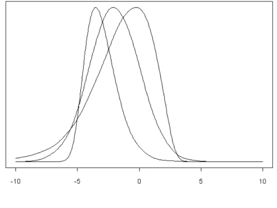
Figure 1. Distributions for different values of µ,

σ

and

λ

Given an estimate of the parameters

µ

,

σ

and

λ

,4 the probability that

α

_i is positive can be easily computed by Monte-Carlo integration.5 Because this estimated probability is a non-linear function of the estimated parameters, it would be very difficult to derive the corresponding sampling distribution. An approximation to this distribution is obtained by using a bootstrap procedure. Bootstrap samples can be generated by drawing with replacement from the whole sample of individuals. Then, for each bootstrap

4

As in Train (1998), the simulated maximum likelihood estimator is also used.

5

The GAUSS built-in normal random number generator was used to draw random numbers from the estimated distribution.

sample, the parameters of the model are re-estimated, and a new estimated probability is computed. Given a large enough number of bootstraps, an approximation to the distribution of the estimator of the probability of interest is obtained.

3. Data Description

In this section, the data set is briefly presented. The province of KwaZulu-Natal lies in the north-eastern corner of the Republic of South Africa. It is a region of extreme natural diversity, boasting lagoons, coral reefs, mountains and some of Africa’s oldest game reserves. The four game reserves that are the focus of this empirical application (Hluhluwe, Umfolozi, Mkuzi and Itala Game Reserves) are administered by the KwaZulu-Natal Parks Board (KNPB), an organization that is responsible both for the reserves’ protection and enhancement and also for providing facilities and accommodation for visitors.

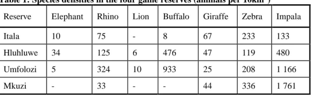
The four reserves are relatively different in the game-viewing experience they afford visitors. Table 1 shows some estimates of the species densities to be found in each of the parks. Households visit the reserves for a number of reasons; Umfolozi is the largest and possibly wildest of the four reserves, Hluhluwe is the only park in which there is a reasonable chance of seeing large herds of elephant, whilst Mkuzi boasts the greatest diversity of bird species. Further, game-viewing is not a science, one day visitors may have marvellous views of animals, the next they may spend a whole day without seeing anything.

Table 1: Species densities in the four game reserves (animals per 10km2)

Reserve Elephant Rhino Lion Buffalo Giraffe Zebra Impala

Itala 10 75 - 8 67 233 133

Hluhluwe 34 125 6 476 47 119 480

Umfolozi 5 324 10 933 25 208 1 166

Mkuzi - 33 - - 44 336 1 761

Source: Extrapolated from KNPB game counts

Since the reserves are relatively remote (the average travel time to a reserve in the dataset is 3.2 hours) and the best time for viewing wildlife is at dawn and at dusk, the vast majority of visitors spend at

least one night in the reserve. Thus, the KNPB provides a range of accommodation types in each of the reserves.

A sample of 1,000 trips made by residents of KwaZulu-Natal province between August 1994 and August 1995 was collected from data stored on the KNPB reservations database. The database indicated each household’s choice of reserve and accommodation. The database was also used to determine which other reserve-accommodation combinations would have been available to a household when making the choice (some accommodation types may already have been booked by other parties or have been unavailable due to maintenance activities). It was also possible to determine exactly how many units of these alternative reserve-accommodation options would be needed to house the party and to calculate the cost they would have paid if they had chosen that option.

Geographical information systems (GIS) were employed to calculate accurate ‘door to park gate’ travel costs (and travel times) using the actual road network and accounting for differences in road speed and fuel efficiency on different types of roads.

Socio-economic characteristics of the households were collected using aggregate GIS data on the smallest unit of the South African census (the enumerator area). Definition and average values for the variables used in this study are provided in Table 3. A more detailed description of the data and the construction of the dataset are provided in Day (1998).

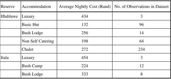
Table 2. Reserve-accommodation choices of chosen reserve-accommodation options

Reserve Accommodation Average Nightly Cost (Rand) No. of Observations in Dataset

Hluhluwe Luxury 434 3

Basic Hut 132 96

Bush Lodge 256 14

Non Self Catering 198 64

Chalet 272 234

Itala Luxury 454 3

Bush Camp 224 12

Non Self Catering 193 1 Chalet 251 158 Mkuzi Cottage 214 76 Basic Hut 134 40 Bush Lodge 255 8 Tent Chalet 157 20 Umfolozi Luxury 468 3 Cottage 223 24 Basic Hut 153 129 Bush Camp 207 26 Bush Lodge 270 13 Chalet 227 68 Total 1 000 Source: KNPB

Table 3. Variables used in the regression analysis

Variable Description Mean Value for Chosen

Option Travel Cost Costs of petrol from households journey to and from

the reserve

R51* Accommodation Cost Total cost to household for accommodation R466* Total Cost Travel cost + Accommodation Cost R517* Hluhluwe Dummy variable for Hluhluwe Reserve taking on a

value of 1 if this option is in Hluhluwe and 0 otherwise

0.42

Itala Dummy variable for Itala Reserve taking on a value of 1 if this option is in Itala and 0 otherwise

0.18

Mkuzi Dummy variable for Mkuzi Reserve taking on a value of 1 if this option is in Mkuzi and 0 otherwise

0.14 Umfolozi Dummy variable for Umfolozi Reserve taking on a

value of 1 if this option is in Umfolozi and 0 otherwise

0.26

4. The Estimated Models and Results

The model presented in section 2 is applied to a unique data set that records details of trips made by domestic households of the KwaZulu-Natal province of South Africa. While a conditional logit (CL) model and an RPL model are estimated in subsection 4.1, in subsection 4.2, besides a conditional logit (CL), a nested logit model approximated by an RPL model (ANL) is estimated, as well as a RPL model, where all the coefficients are random, i.e., the nest-specific dummy coefficients and the total cost coefficient. This last model is identified in the paper as Full Random Parameters Logit (FRPL).

4.1. The estimated model and results: the first data set

In the case of the first data set, we considered individuals’ park choice as a function of observed accommodation costs. Accommodation costs for nonchosen parks were obtained by calculating costs averages over the accommodations available in that specific park.

4.1.1. The Conditional Logit Model

The results of the estimated conditional logit model are presented in Table 4. Park1 (Hluhluwe), Park2 (Itala), and Park4 (Umfolozi) are choice specific indicators for three of the four parks, and AC stands for accommodation costs. The choice specific indicators capture the influence of all characteristics of each park that were not considered as regressors in the model. The highest coefficient is for Park1 (1.6373), indicating the preference of individuals for this park over the other parks. Because all estimated choice specific indicators coefficients are positive, it seems that if accommodation costs were the same in all parks, the least preferred park would be Park 3 (Mkuzi).

Table 4: The Conditional Logit Model - CL Variables Coefficients Standard Errors AC -8.8282*** 0.4950

Park1 1.6373*** 0.1197

Park2 1.2293*** 0.1407

Log-likelihood: -1085.46 ***1% significance level

The sign of the coefficient on accommodation costs is negative as expected. All the coefficients in the conditional logit model are significant at the 1% significance level.

4.1.2. The Random Parameters Logit Model (normal)

The variables considered in the conditional logit model were also included in the RPL model. In the RPL model with a normal distribution for the coefficient of a given variable, the mean and the standard deviation of this distribution are estimated. In Table 5, the estimates of the fixed coefficients of the variables Park1, Park2 and Park4, are presented, as well as estimates of the mean, µ, and the standard deviation, σ, of the normal distribution of the coefficient on accommodation costs.

Table 5: The Random Parameters Logit Model (normal) - RPL (normal) Variables Coefficients Standard Errors AC µ -12.0567*** 1.0070

σ

11.1091*** 1.6214 Park1 1.9098*** 0.1438 Park2 1.4437*** 0.1584 Park4 0.9451*** 0.1410 Log-likelihood: -1077.58 ***1% significance level

The coefficients for the Park variables, which are fixed, have similar interpretations to the ones given in the conditional logit model (Table 4). The estimated distribution for the coefficient on the accommodation cost variable is

α

i

~

N

(

−

12

.

0567

,

(

11

.

1091

)

2

)

.

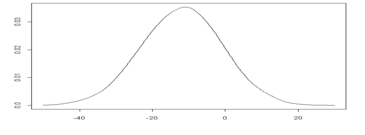
Figure 2. Estimated normal distribution for αi

The estimate of the mean is negative as it should be for rational individuals. The assumption of a non-random parameter can be tested by a likelihood ratio test that compares the likelihood function for this model with the value for the likelihood function in Table 4. The resulting statistic, LR=15.77, is greater than the critical value for a chi-squared with 1 degree of freedom at the 5% significance level. Therefore, the non-random parameter assumption is clearly rejected.

According to the RPL model presented in section 2, the probability that the cost coefficient is positive in the sample represents the share of individuals in the population with nonrational choice behavior. If

α

i is normally distributed with mean µ and standard deviation

σ

, this probability can be

computed as

[

] [

]

_







_>

₋

=

>

+

=

>

σ

µ

σ

µ

α

i

0

Pr

z

i

0

Pr

z

i

Pr

,

where

z

j

~ N

(

0

,

1

)

. Given normality, it follows that the estimated probability is

[

]

Pr

[

1

.

085

]

0

.

14

1091

.

11

0567

.

12

Pr

0

Pr

=

>

=







 >

=

>

i i i

z

z

α

.

Therefore, the model estimates that 14% of the individuals in the sample do not behave rationally. However, this estimated probability may be sensitive to misspecification of the underlying distribution function.

4.1.3. The Random Parameters Logit Model (transformed)

In order to account for the possibility of misspecification of the underlying distribution function, we consider a family of distributions, where the normal is a particular case, that is,

α

_i

=

β

_i

+

λβ

_i2, where

β

i ~

N

(

µ

,

σ

2

)

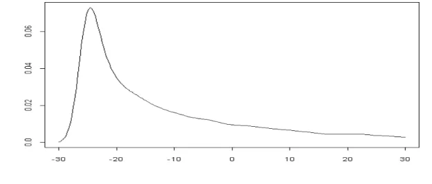
. The results are shown in Table 6.

Table 6: The Random Parameters Logit Model (Transformed) - RPL (transformed) Variables Coefficients Standard Errors AC µ -25.1669*** 2.6870

σ

32.5288*** 4.1838 λ 0.0098*** 0.0009 Park1 1.9641*** 0.1537 Park2 1.4866*** 0.1689 Park4 1.0252*** 0.1463 Log-likelihood: -1069.60 *** 1% significance level

At the estimated values of the parameters it follows that

α

_i

=

β

_i

+

0

.

0098

β

_i2 , where

)

)

5288

.

32

(

,

1669

.

25

(

~

−

2

β

_i

N

.

Figure 3. Estimated general distribution for αi

In this case, the results obtained for the Park variables coefficients are similar to those obtained previously. Regarding the accommodation cost coefficients, the estimated values for µ and

σ

in the RPL (transformed) are quite different from the normal distribution case (see Table 5). However, these are not comparable because the new mean and standard deviation of the distribution are now a function of µ,

σ

_and

λ

. The estimated

λ

is significant at the 1% significance level. The normality assumption can also be tested by a likelihood ratio test that compares the value of the log-likelihood function for this model with the one in Table 5. The value is LR=15.96, greater than the critical value for a chi-squared with 1 degree of freedom at the 5% significance. Therefore, the normality assumption, that is,

λ

=

0

, is clearly rejected.

Given that the distribution in the RPL (transformed) is unknown, we cannot use standard statistical tables to determine the percentage of nonrational individuals in the sample. Thus, by Monte-Carlo integration, simple statistics can be easily derived by drawing large number of times from the estimated distribution. The resulting mean and standard deviation of

α

_iare -8.62 and 22.05, respectively. The share of individuals behaving nonrationally in the sample in this more flexible context can be computed in a similar manner by drawing a large number of times from the estimated distribution and

computing the percentage of draws that gives a positive

α

i . The resulting estimate gives a value of 23%,

which is larger than in the normal case. Thus, the normality assumption, in the case of this paper, underestimates nonrational behavior in the sample.

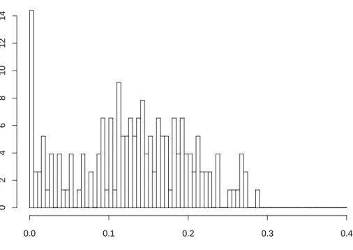
So far, the reported estimated probability followed directly from the point estimates of the parameters. A confidence interval for the proportion of individuals that behave nonrationally can be constructed by an approximation to the distribution of the estimator of the unknown probability using a bootstrap procedure. Each bootstrap sample is generated by drawing with replacement from the whole sample of individuals. For each bootstrap sample, the model is re-estimated and a new probability is computed following the procedure described above. If we use a sufficient large number of bootstrap samples the set of generated estimated probabilities can be used to compute a bootstrap confidence interval. In Figures 4 and 5 we present an histogram of the bootstrap probabilities assuming the normal distribution and the more general distribution estimated above for the accommodation cost coefficient, respectively.

Figure 4. Histogram of bootstrap probabilities assuming a normal distribution

For the general distribution, the histogram clearly suggests that, with a high degree of confidence, the probability of nonrational behavior is large. In fact, the distribution of

α

_i is concentrated around 0.23, and well away from zero.

0.0 0.1 0.2 0.3 0.4 0 2 4 6 8 10 12 14

Figure 5. Histogram of Bootstrap Probabilities assuming the general distribution

The same does not hold when the assumed distribution is normal. As the likelihood ratio test reported (LR=15.96) already suggested, the general distribution was preferred. It is also possible to look at the histogram of the bootstrap values of

λ

to confirm that the normal distribution is not adequate. The distribution of

λ

is concentrated around 0.1, and well away from zero, confirming the results obtained above by the LR test.

0.0 0.1 0.2 0.3 0.4

0

5

10

Figure 6. Histogram of Bootstrap

λ

In order to examine the explanatory power of the models presented, one should examine the likelihood ratio index. The likelihood ratio index is 0.0058 for the standard logit model, 0.1673 for the RPL (normal), and 0.1735 for the RPL (transformed). Thus, the RPL (transformed) has a better explanatory power than the RPL (normal), which has a better explanatory power than the conditional logit model does.

4.2. The estimated model and results: the second data set

The second data set includes not only accomodation costs, but also travel costs. The choices involve, both parks and accommodations in each park. Table 7 presents the results of the Conditional Logit Model (CL) and the Approximated Nested-Logit (ANL). The coefficients of the park variables as well as the coefficient of total cost are significantly different from zero. The coefficient of total cost has the expected negative sign. The nested structure versus the conditional logit one can be tested by computing the likelihood ratio test that compares the value of the likelihood function for the CL and the ANL models. The value of the likelihood ratio test is LR=6.68, which is smaller than the critical value for a chi-squared with three degrees of freedom at the 5% significance level. Therefore, at 5%, the conditional

logit structure cannot be rejected. However, the value of the likelihood ratio test is marginally larger than the critical value for a chi-squared with three degrees of freedom at the 10% significance level. Therefore, at 10%, the conditional logit structure is rejected in favor of the nested one.

Table 7. Conditional Logit (CL) and Approximated Nested-Logit (ANL) Conditional Logit Approximated Nested-Logit Variables Coefficients St. Error Coefficients St. Error Total Cost -2.8994*** 0.1808 -2.9864*** 0.1891 Park1 0.9998*** 0.0976 µ -- -- 0.9970*** 0.0992 σ -- -- 0.2918 0.7217 Park2 0.4222*** 0.1157 µ -- -- 2.0072 1.9432 σ -- -- 3.9919* 2.3220 Park4 0.4294*** 0.1044 µ -- -- 0.4123*** 0.1216 σ -- -- 0.1894 0.8425 Log-likelihood: -2 573.33 -2 569.99 *** 1% significance level * 10% significance level

As the results are not strong enough in favor of the nested structure, we test for rationality in the context of both a nested and a nonnested structure. Using the nonnested structure, and proceeding as we did with the first data set, we compare the results obtained in the CL model with those in the RPL model, where the random coefficient of the total cost variable is distributed as a normal. As it is clear from Table 8, the standard deviation of the distribution of the coefficient of the total cost variable is not significant, suggesting that this coefficient does not vary randomly. As with the first data set, the transformed RPL model is also estimated. However, the results show that the estimated λ is not significant (see Table 8). Therefore, nonrationality is rejected.

Table 8. RPL (normal) and RPL (transformed) RPL (normal) RPL (transformed) Variables Coefficients St. Error Coefficients St. Error Total Cost µ -2.8998*** 0.1808 -2.9005 6.0297 σ 0.0266 0.2748 0.0256 0.2934 λ -- -- -0.0002 0.7159 Park1 1.0014*** 0.0976 0.9996*** 0.0976 Park2 0.4207*** 0.1158 0.4214*** 0.1157 Park4 0.4314*** 0.1044 0.4292*** 0.1044 Log-likelihood: -2 573.33 -2 573.33 *** 1% significance level

Alternatively, using the nested structure, we compare the results in the ANL model with those in the full random parameters logit (FRPL) model, where in addition to the random cost coefficient, the coefficients of the three dummies for each park are also normally distributed. Thus, all the coefficients are random in this model. These results are presented in Table 9. Computing the likelihood ratio test, the value obtained is LR=0.04 which is smaller than the critical value for a chi-squared with one degree of freedom at 5% significance level. Therefore, nonrationality is rejected in this model, confirming the previous result.

Table 9. Approximated Nested-Logit (ANL) and FRPL (normal)

Approximated Nested-Logit (ANL) FRPL (normal) Variables Coefficients St. Error Coefficients St. Error Total Cost -2.9864*** 0.1891 µ -- -- -2.9864*** 0.1891 σ -- -- 0.0543 0.2693 Park1 µ 0.9970*** 0.0992 0.9970*** 0.0993 σ 0.2918 0.7217 0.2918 0.7216 Park2 µ 2.0072 1.9432 2.0072 1.9432 σ 3.9919* 2.3220 3.9919* 2.3219 Park4 µ 0.4123*** 0.1216 0.4123*** 0.1216 σ 0.1894 0.8425 0.1894 0.8419 Log-likelihood: -2 569.99 -2 569.97 *** 1% significance level * 10% significance level 5. Conclusions

In order to use the estimates of individuals’ willingness to pay for policy purposes, these willingness to pay measures should be supported by an underlying rational preference structure, according to the neoclassical theory of preferences.

In the context of an estimated RPL choice model of recreational demand for the four game reserves of the KwaZulu-Natal province in South Africa, a test on the existence of an underlying rational preference structure is performed. Moreover, by introducing flexibility into the model, it is possible to identify nonrational behavior in the sample, distinguishing eventual biases on choice behavior caused by the particular shape of the distribution chosen to represent the random coefficient from genuine nonrational choice behavior. Two data sets extracted from the original database were examined. The first one attempts to explain the park choice as a function of the observed accommodation costs, where costs gross averages were used for the nonchosen parks. In the second one, travel costs were also introduced. In

this case, the choices involve both parks and accommodations in each park. The results obtained with each model were radically different. While using the first data set significant nonrational behavior was identified, in the second data base nonrational behavior was not found. Therefore, by improving the data, apparent nonrationality can be eliminated and welfare analysis may be safely conducted. The bias on choice behavior caused by the nature of the data can be clearly identified following the procedure proposed in this paper. This is in contrast with previous work in the literature, where rational behavior is usually assumed a priori.

References

Davidson, R., J. G. MacKinnon, 1993, Estimation and Inference in Econometrics, Oxford University Press.

Hanemann, W. M., 1984, Discrete/Continuous Models of Consumer Demand, Econometrica 52, 541-561. Nunes, L., M. Cunha-e-Sá, and M. Ducla-Soares, 1998, “Testing for Rationality: The Case of

Discrete-Choice Data.”, Economics Letters, Vol. 60.

MacFadden, D., and K. E. Train, 1997, “Mixed MNL Models for Discrete Response”, unpublished manuscript.

Train, K. E., 1998, “Recreation Demand Models with Tastes Differences over People”, Land Economics, 74 (2):230-39.

Ichimura, H., and T.S.Thompson, 1998, “Maximum Likelihood Estimation of a Binary Choice model with Random Coefficients of Unknown Distribution”, Journal of Econometrics, Vol. 86, 2.