Characterization of the Deformation Behaviour of Mould Slag Inclusions During Hot Rolling

(1)

Characterization of the Deformation Behaviour of Mould

Slag Inclusions During Hot Rolling

Guilherme Melo

Master Dissertation

FEUP Supervisor: Prof. Fernando Jorge Lino Alves Tata Steel Supervisor: Laurens-Jan Pille

Integrated Master in Mechanical Engineering

(2)

(3)

iii

(4)

(5)

v

Abstract

The present work aimed at furthering the characterization of the chemo-thermo-mechanical phenomena occuring during the hot-rolling of steel containing inclusions resulting from the mould slag in continuous casting.

To do so, artificial inclusions were embedded into powder metallurgy cylinders, which were fitted into steel slabs and rolled according to different schedules in a lab-scale hot strip mill. Different preparation conditions of the inclusions (fluorine and sodium content) and differences in the rolling process (soaking time, thickness reduction) ensured that several combinations of parameters were tested. The rolled inclusions were retrieved from the slabs in samples corresponding to longitudinal sections and characterized using optical and electron microscopy techniques.

Additionally, a finite element model of the lab-scale hot rolling process was developed to complement the interpretation of the results.

It was observed that a significant change in inclusion shape occurred between the rolling schedules with 2 and 3 passes. Evolutions in the relative plasticity index and aspect ratio of the inclusions were also displayed with varying depths within the slab and thickness reduction applied. No influence of the composition or soaking times was observed in the inclusion shape. It was also concluded that the methodology used to produce variable F/Na contents resulted in different phases observed, where the poor F/Na inclusions presented both cuspidine and wollastonite as crystalline phases, while the rich F/Na displayed cuspidine as the single crystalline phase present.

Finally, it was observed that wollastonite was consistently found in elongated blocks in the rolling direction, whereas the cuspidine morphology changed significantly between globular and dendritic structures depending on the depth within the slab and additional phases present. For the most deformed inclusions, cuspidine also presented a change in morphology in the longitudinal direction, from a dendritic to a globular structure.

(6)

(7)

vii

Caracterização da Deformação de Inclusões Provenientes de Fluxos

de Cobertura Durante Laminagem a Quente

Resumo

O presente trabalho teve como objetivo aprofundar a caracterização dos fenómenos químico-termo-mecânicos occorrentes durante o processo de laminagem a quente de aço com inclusões provenientes da escória criada pelos fluxos de cobertura no processo de vazamento contínuo. Para tal, foram intruduzidas inclusões artificiais em cilíndros criados por pulverometalurgia, os quais foram inseridos em blocos de aço e sujeitos a diferentes sequências de laminagem a quente num laminador à escala laboratorial. A variação das condições de preparação das inclusões (relativamente ao conteúdo de sódio e flúor) e as diferenças no processo de laminagem (tempo de pré-aquecimento, redução de espessura) promoveram que diferentes combinaçoes de parâmetros fossem testadas. As inclusões laminadas foram recuperadas dos blocos de aço em amostras correspondentes a secções longitudinais e caracterizadas usando microscopia ótica e eletrónica.

Adicionalmente, foi desenvolvido um modelo de elementos finitos do processo de laminagem a quente à escala laboratorial com o objetivo de auxiliar a interpretação dos resultados.

Foi observado que ocorreu uma alteração considerável na forma das inclusões entre as sequencias de laminagem com 2 e 3 passagens. Foram também observadas evoluções do índice de plasticidade relativa e razão de aspeto das inclusões com a variação da profundidade no bloco de aço e redução de espessura aplicada. Não foi possível detetar influências da composição ou tempo de pré-aquecimento na forma final das inclusões.

Foi também concluído que a metodologia empregue para produzir duas variações do conteúdo de flúor e sódio resultou em fases diferentes observadas, sendo que as inclusões pobres em F/Na apresentaram cuspidine e wollastonite como fases cristalinas, enquanto que as inclusões ricas em flúor e sódio revelaram apenas cuspidine como a única fase cristalina presente.

Por fim, observou-se que a wollastonite foi consistentemente encontrada sob a forma de blocos alongados na direção de laminagem, enquanto que a cuspidine apresentou mudanças consideráveis na sua morfologia, entre estruturas globulares e dendríticas, dependendo da profundidade no bloco de aço e das restantes fases presentes. Nas inclusões mais deformadas, a cuspidine apresentou ainda uma alteração da sua morfologia na direção longitudinal, mudando de uma estrutura dendrítica para uma estrutura globular.

(8)

(9)

ix

Acknowledgements

I would fistly like to thank Sido Sinnema for the oportunity provided for the realization of the internship in the CRC, which led to the present work.

Secondly, I would like to thank Laurens-Jan Pille,Wouter Tiekink and Fernando Jorge Lino Alves for the guidance provided in their supervison, whithout wich the present work would not have been possible.

I would also like to thank James Small and Frank van der Does for all the help and expertise provided during the microscopy techniques used. Additionally, I would like to thank Enno Zinngrebe for the input provided for the chemical aspects of the present thesis.

Regarding the work conducted within the Innovation Centre at Tata Steel IJmuiden, I am especially thankful for the support, guidance and work environment provided by Edwin Swart as well as for the crucial help provided by Martin Sadhinoch during the development of the FE model. Moreover, I would like to thank Peter Gelten for the help provided regarding the material model used.

I would like to thank all remaining personel in the Ceramics Research Centre and Innovation Centre at Tata Steel IJmuiden for the amicable and pleasant work environment provided during the internship.

I would like to thank the Faculty of Engineering of the University of Porto for the learning experience provided.

I would also like to express my gratitude to my parents, for the unconditional support and constant interest in my studies.

Finally, I would like to thank both Tata Steel and the Erasmus program for the financial support provided.

(10)

(11)

xi

List of Symbols

A - area of the inclusion’s section a - contact length

c - specific heat of the rolled material

cx - fitting coefficients of the Siciliano model

epa - strain rate

eps - deformation strain

E1 - Young modulus of the cylinder in the Hertzian contact situation

E2 - Young modulus of the slab in the Hertzian contact situation

E* - combined Young modulus in the Hertzian contact situation F - applied force in the Hertzian contact situation

f - composition-based factor in the Siciliano model FS - field strength

ℎ - average convective heat transfer coefficient ha - convection heat transfer coefficient

hc - contact conductance between the slab and the roll

k - thermal conductivity of the rolled material kair - conductivity of the air

ks - shear yield stress

L - length of the slab Li - initial slab length

lf - length of the inclusion after rolling

Ln - normalized final slab length

m - sticking friction factor MAR - maximum aspect ratio MFS - mean flow stress

n - normal direction to the surface boundary during hot rolling NAR - normalized aspect ratio

- average Nusselt number for x=L

P

- contact pressure

pmax - maximum contact pressure

Pr - Prandtl number for the air

q - heat flux per unit area that crosses the surface from the slab to the roll qf - rate of generated heat by friction on the contact surface during hot rolling

ReL - Reynolds number for x=L

RPI - relative plasticity index

rpl - heat flux generated per unit of volume due to plastic deformation during hot rolling Rx - cooling rates applied in the slag characterization tests

R1 - radius of the cylinder in the Hertzian contact situation

R2, - radius of the slab in the Hertzian contact situation

R* - combined radius

S - Stefan–Boltzmann constant SI - shape index of the inclusion T - temperature

(14)

xiv Tb - temperature of point b, in the roll

Tf - final slab thickness

tfmax - maximum inclusion thickness after rolling

tfnorm - normalized inclusion thickness after rolling

Tg - glass transition temperature Ti - initial slab thickness

Tl - liquidus temperature

Troll - work-roll surface temperature

T∞ - ambient temperature

u - velocity component along x direction

u∞ - relative speed of the air in relation to the slab

v - velocity component along y direction w - velocity component along w direction

- average final slab width Wi - initial slab width

[X] - fractions of each chemical element X in the Siciliano model x - rolling direction during hot rolling

y - transverse direction during hot rolling z - thickness direction in during hot rolling

αR - mass proportional damping coefficient in the Rayleigh damping method

βR - stiffness proportional damping coefficient in the Rayleigh damping method

Δv - relative tangential velocity between the slab and the roll ̅ - average inclusion strain

̅ - average steel strain - strain rate vector

η - fraction of friction heat transferred to the slab during hot rolling ηp - fraction of plastic work converted to heat

λ - surface emissivity

µ

- coefficient of friction ν - dynamic viscosity of the air

ν1 - Poisson coefficient of the cylinder in the Hertzian contact situation

ν2 - Poisson coefficient of the slab in the Hertzian contact situation

ξ - normalized contact length ρ - density of the rolled material

- stress vector

τc - critical shear stress value

(15)

xv

List of Abbreviatures

BEI (or BSE) - back-scattering electron imaging BF - blast furnace

BOF - basic oxygen furnace BOP - basic oxygen process BOS - basic oxygen steelmaking

CCT - continuous cooling transformation CIP - carbonyl iron powder

EAF - electric arc furnaces

EDS - energy dispersive X-ray spectroscopy ESEM - environmental scan electron microscopy FE – finite elements

HIP - hot isostatic pressing

LVSEM - low voltage scan electron microscopy NMI - non metallic inclusions

SEN - submerged entry nozzle MP - mould powder

PM - powder metallurgy

PVD - physical vapour deposition SEM - scan electron microscopy

TEM - transmission electron microscopy TTT - time temperature transformation

(16)

(17)

xvii

List of Figures

Figure 1 - Example of the Griffe Laminée defect ... 3

Figure 2 - Example of the Split Flanges defect ... 4

Figure 3 - Schematic representation of the BOF and continuous casting process flow at Tata Steel IJmuiden ... 5

Figure 4 - Schematic representation of the continuous casting process ... 6

Figure 5 - Detail of the continuous casting process (left) and respective mould powder layers in the mould (right) ... 7

Figure 6 - The coefficient of friction as a function of velocity for two different steel grades ... 8

Figure 7 - The coefficient of friction as a function of thickness reduction for different temperatures ... 9

Figure 8 - Schematic representation of the neutral point and different slip regions ... 10

Figure 9 - Inhomogeneous deformation of material between rolls. Shaded areas are non-plastic regions ... 10

Figure 10 - SiO44-_{tetrahedron (left) and a silicate network (right) ... 11}

Figure 11 - Role of sodium and calcium oxides in modifying the silica network ... 12

Figure 12 - Phase diagram for the SiO2-CaO-Na2O ternary system ... 14

Figure 13 - Phase diagram for the SiO2-CaO-Na2O-CaF2 quaternary system ... 15

Figure 14 - Different types of inclusions in hot-rolled steel: (a) undeformed ‘hard’ inclusion, (b) brittle broken crystalline inclusion, (c) hard inclusion cluster (d) brittle–ductile multiphase complex inclusion and (e) ductile elongated inclusion. The scale in figures vary from few microns to tens of microns ... 16

Figure 15 - SEM picture of a multiphase Non Metallic Inclusion ... 17

Figure 16 - Measured and computed onset temperatures as a function of heating rate (ϕ) for peak 1 (cuspidine) during devitrification of mould slag A ... 18

Figure 17 - Temperature (yy axis) as a function of processing time (xx axis) for the different rolling stations (V1 through V6) at the centre of the slab (kern, red) and at the surface of the slab (oppervlak, blue) ... 19

Figure 18 - Schematic drawing of the iron decomposition process ... 24

Figure 19 - Hot isostatic pressing system representation ... 25

Figure 20 - Different possible electron behaviour as a base for SEM image modes (left) and X-Ray emission mechanism as the base for the EDS mode (right) ... 26

Figure 21 - Schematic representation of the production of the samples studied in the first stage. Indexed numbers indicate the slab numbers that result from the alternative processing routes, as can be consulted in Table 3-4 ... 29

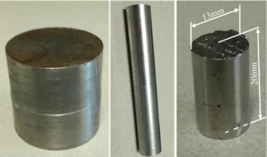
Figure 22 - Graphic representation of the (a) artificial inclusions, (b) PM cylinder with embedded artificial inclusions and (c) steel slab with shrink fitted PM cylinder ... 30

(18)

xviii Figure 24 - Shaping step (left) and SEM image of the artificial inclusions after the

shaping and final sieving steps (right) ... 31 Figure 25 - Powder metallurgy cylinders after HIP and machining (left, centre) and after

cutting (right) ... 32 Figure 26 - Slabs 1 (lower left corner), 2 (lower right corner) and 3 (top) after hot rolling.

PM cylinders visible in the centre of the slabs ... 33 Figure 27 - Struers Accutom-5 used in the sample cutting process ... 34 Figure 28 - Representation of the expected deformation of the rolled cylinders (not to

scale) ... 34 Figure 29 - Struers PolyFast carbon-filled phenolic resin (left) and Struers Protonpress

10 (right) used in the sample mounting ... 34 Figure 30 - Struers Tegramin-30 used in the automated sample grinding and polishing

steps ... 35 Figure 31 - Mosaic created with 50x optical microscopy images. Samples taken from the

85% reduction slabs ... 37 Figure 32 - Detail of sample from slab 8 (top) and 12 (bottom) created with 50x optical

microscopy images. Relevant inclusions identified with capital letters above ... 38 Figure 33 - Detail of the sample from slab 2 created with 50x optical microscopy images.

Boundary between the steel slab and the powder metallurgy cylinder highlighted ... 38 Figure 34 - Example of the results of the measurements conducted on the inclusions of

slab 8 during optical microscopy ... 39 Figure 35 - Examples of individual BSI images, resulting from the SEM testing ... 39 Figure 36 - Example of the oval shape displayed in the 20% reduction inclusions.

Example taken from slab 1, inclusion A. Rolling direction from left to right ... 40 Figure 37 - Example of the oval shape displayed in the 40% reduction inclusions.

Example taken from slab 2, inclusion C. Rolling direction from left to right ... 40 Figure 38 - Example of the drop-like shape displayed in the 85% reduction inclusions.

Examples taken from slab 8, inclusions A, B, C and D. The thin part of inclusions C and D is not fully displayed in the picture due to size restrictions. Rolling direction from left to right ... 40 Figure 39 - Example of the strain rate dependency of the elasto-plastic response of the

slab material for a fixed temperature of 1200°C ... 47 Figure 40 - Example of the temperature dependency of the elasto-plastic response of the

slab material for a fixed strain rate of 10 [s-1_{] ... 47}

Figure 41 - Rolling force (left) and displacement curves of the strip (right) for different damping factors ... 48 Figure 42 - Work-roll partitioning (left) and mesh (right) used to reduce the number of

elements ... 53 Figure 43 - Detail of the transition zones with triangular elements (left) and element size

ratio between the roll and the strip (right) ... 53 Figure 44 - Schematic representation of the Hertzian contact situation ... 54

(19)

xix Figure 45 - Analytical and finite element solutions determined by Gillebaart (2011) for

the pressure distribution throughout the contact length in the Hertzian contact problem ... 55 Figure 46 - Predicted temperature evolution at different slab depths (as a percentage of

the initial slab thickness) during the one-rolling step, 40% thickness reduction, lab-scale hot rolling FE simulation ... 56 Figure 47 - Predicted temperature evolution at different slab depths (as a percentage of

the initial slab thickness) during the single-step, lab-scale hot rolling FE simulations (20% and 40% thickness reduction) ... 57 Figure 48 - Contact zones for the single-step, lab-scale hot rolling FE simulations (20%

and 40% reduction ... 57 Figure 49 - Heat transfer during hot rolling for the 40% reduction hot rolling simulations.

Legend in [kW/m2_{] units with lower bound set at 500 to highlight the}

conduction in the contact zone ... 58 Figure 50 - Temperature gradient during hot rolling for the 20% reduction hot rolling

simulations. Legend in Kelvin [K] units with lower bound set at 1473 (=1200°C) to highlight only the temperature increase above the initial conditions ... 58 Figure 51 - Temperature gradient during hot rolling for the 40% reduction hot rolling

simulations. Legend in Kelvin [K] units with lower bound set at 1473 (=1200°C) to highlight only the temperature increase above the initial conditions ... 59 Figure 52 - Predicted temperature evolution at different slab depths (10mm and 20mm

correspond to 5% and 10% of the initial slab thickness, respectively) during the first rolling step (15% thickness reduction) of the plant-scale, hot rolling FE simulations conducted by Serajzadeh et al. ... 60 Figure 53 - Experimental surface temperature measurements at the entry (In) and exit

(Out) of the lab-scale hot rolling mill for the single-pass, 20% reduction experiments ... 61 Figure 54 - Predicted temperature evolution at different slab depths (as a percentage of

the initial slab thickness) during the two-rolling step, 60% thickness reduction, lab-scale hot rolling FE simulation ... 62 Figure 55 - Predicted temperature evolution at different slab depths (as a percentage of

the initial slab thickness) during the three-rolling step, 85% thickness reduction, lab-scale hot rolling FE simulation. Measured surface temperature plotted for the slabs in the rolling trials ... 62 Figure 56 - Predicted and measured temperature variations during a 6-roughing stand,

hot rolling process. FE model considering the thermo-mechanical-metallurgical response of a low-carbon steel ... 63 Figure 57 - Finite Element results (left) and experimental results (right) for the rolling

force evolution throughout the single-pass, 20% reduction rolling schedule ... 64 Figure 58 - Finite Element results (left) and experimental results (right) for the rolling

force evolution throughout the first pass in the 60% reduction rolling schedule ... 64

(20)

xx Figure 59 - Finite Element results (left) and experimental results (right) for the rolling

force evolution throughout the second pass in the 60% reduction rolling schedule ... 65 Figure 60 - Relative displacements of a column of elements for the two single-pass hot

rolling simulations (left) and for the 3-pass, 85% thickness reduction hot rolling simulation (right). Direction yy displayed as a percentual proportion to the final thickness to allow a comparison between the slabs ... 66 Figure 61 - Relation between the normalized and the maximum aspect ratios.

Nomenclature of the subtitle indicates the slab number (1-16) and its respective thickness reduction (%), the F and Na content (Poor/Rich) and the soaking time (Low/High) ... 68 Figure 62 - Influence of thickness reduction on the normalized aspect ratio of the

inclusions ... 69 Figure 63 - Evolution of the standard deviation for the normalized aspect ratio

measurements with thickness reduction ... 69 Figure 64 - Influence of depth on the maximum aspect ratio of the inclusions ... 70 Figure 65 - Influence of depth on the normalized aspect ratio of the 85% reduction

inclusions ... 70 Figure 66 - Influence of depth on the final length of the 85% reduction inclusions ... 71 Figure 67 - Plastic equivalent strain after rolling for the 40% (left) and 85% (right) hot

rolling simulations. Deformed slab profiles for each situation presented above each curve ... 71 Figure 68 - Influence of thickness reduction on the shape index of the inclusions ... 72 Figure 69 - Deformation of inclusions located in the centre of the modelled slab for a low

reduction (light) multi-pass rolling scheme up to 20% thickness reduction (a) and for a higher reduction (high) multi-pass rolling scheme up to 42% thickness reduction (b) ... 73 Figure 70 - Hard Al2O3 inclusion behaviour during multi-pass cold rolling operations.

Initial inclusion diameter of 20 µm ... 73 Figure 71 - Evolution of the relative plasticity index for inclusions located in the centre

of the slab during the hot rolling process for the high reduction pass FE simulations conducted by Luo and Ståhlberg (2001) ... 74 Figure 72 - Evolution of the relative plasticity index with thickness reduction for the

experimental data ... 75 Figure 73 - Relative plasticity index (indicated as “index”) evolution with the depth of

the layer at which the inclusion is located (depth decreases for higher numbers) and the number of rolling passes ... 76 Figure 74 - Relative plasticity index evolution with the depth of the inclusion for the 60%

thickness reduction inclusions ... 76 Figure 75 - Relative plasticity index evolution with the depth of the inclusion for the 85%

thickness reduction inclusions ... 77 Figure 76 - Inclusion profile evolution for the last step of a 3-pass rolling schedule with

(21)

xxi Figure 77 - Temperature profile in the middle of the slab at the end of the 1st_{rolling step}

(last stage of the 40% reduction rolling experiments) 2nd_{rolling step (last}

stage of the 60% reduction rolling experiments) and at the end of the 3rd

rolling step (last stage of the 85% reduction rolling experiments) ... 78 Figure 78 - Average Relative Plasticity Index for the inclusions found in each slab. Slabs

grouped by F and Na content (poor/rich) and soaking time (low/high) ... 79 Figure 79 - Average Maximum Aspect Ratio for the inclusions found in each slab. Slabs

grouped by F and Na content (poor/rich) and soaking time (low/high) ... 79 Figure 80 - Section of the stitched BSI images for inclusion A found in the sample

prepared from slab 1 at a depth of 3225µm (20% of the final slab thickness). Rolling direction from left to right ... 83 Figure 81 - Stitched BSI images for inclusions A (middle), B (right) and C (left) in the

sample from slab 2. Inclusions organized (left to right) by increasing depth within the slab. Depths: inclusion C, 274µm (2% of the final slab thickness); inclusion A, 1736µm (14%) and inclusion B, 3136µm (26%) ... 84 Figure 82 - Temperature gradient during hot rolling for the 40% reduction hot rolling

simulations. Legend in Kelvin [K] units with lower bound set at 1173 (= 900°C) to highlight only the slab temperature profile ... 85 Figure 83 - Path of elements chosen for plotting the temperature profile in the beginning

of the contact zone, middle of the contact zone and end of the contact zone ... 85 Figure 84 - Temperature evolution with the depth within the slab for the 40% reduction

hot rolling simulations conducted. Temperature profile taken in the beginning, middle and end of the contact zone. Depths of inclusions A, B and C from slab 2 marked on the curve. Only half the thickness is displayed (symmetry) ... 86 Figure 85 - Stitched BSI image section taken from inclusion A, slab 4 (top) and detail

where the different phases are identified (bottom). Phases present are wollastonite (dark grey), cuspidine (light grey) and the remaining glassy phase (medium grey). Inclusion found at a depth of 1182µm (39% of the final slab thickness) ... 87 Figure 86 - Stitched BSI images for inclusion B of the sample from slab 6. Depth and

length of the inclusion are 2194µm (18% of the final slab thickness) and 866µm respectively. Rolling direction from left to right ... 88 Figure 87 - BSI images taken from inclusion B, slab 6, highlighting the frozen transition

zone between the glassy phase and the crystallized cuspidine ... 88 Figure 88 - BSI image “tail” sections from inclusions B (bottom) and D (top) found in

the samples prepared from slab 8. Inclusions organized (top to bottom) by increasing depth within the slab. Depths: inclusion D, 606µm (20% of the final slab thickness) and inclusion B, 1412µm (47%). Rolling direction from left to right ... 89 Figure 89 - Temperature gradient during the last hot rolling pass for the 85% reduction

hot rolling simulations. Legend in Kelvin [K] units with range set from 1173 to 1323 (=900°C to 1050°C) to highlight only the displayed slab zone temperature profile ... 89

(22)

xxii Figure 90 - Temperature evolution with the depth within the slab for the third pass of the

85% reduction hot rolling simulations conducted. Temperature profile taken in the beginning, middle and end of the contact zone. Depths of inclusions A, B, C and D from slab 8 marked on the curve ... 90 Figure 91 - Detail from the Stitched BSI image from inclusion B, slab 8 where transition

zone between the initial glassy structure, the following dendritic structure, the consequent broken dendrite zone and final globular structure is visible in a single image. A similar behaviour was observed for the remaining inclusions from the same sample, albeit more spread out through the inclusions, limiting its display ... 90 Figure 92 - BSI image of an inclusion taken from slab 7 (60% thickness reduction, rich

Na/F content, low soaking time). Inclusion length of 1028µm. Rolling direction from left to right ... 91 Figure 93 - Powder metallurgy bar with visible layering ... 96 Figure 94 - Thermal cycles initially proposed for the different sample preparations ... 97 Figure 95 - Illustration of the CCT and TTT diagrams and corresponding approaches ... 97 Figure 96 - TTT diagram for slag A (Maldonado et al., 2014), of similar composition to

the MP-B slag ... 98 Figure 97 - Microstructures observed for different thermal cycles applied to the mould

slag. BSE images ... 98 Figure 98 - Graphite crucible used by Pieter Put, 2012 ... 99 Figure 99 - Example of a sample produced by Pieter Put, 2012 ... 99 Figure 100 - Principles behind the proposed mechanical characterization test ... 100

Appendices

Figure A1 - Steel slab before hot rolling. PM cylinder visible in the centre of the slab ... 105 Figure A2 - Steel slab after the 20% thickness reduction lab scale hot rolling scheme. PM

cylinder visible in the centre of the slab. Example taken from slab 5 ... 105 Figure A3 - Steel slab after the 40% thickness reduction lab scale hot rolling scheme. PM

cylinder visible in the centre of the slab. Example taken from slab 12 ... 106 Figure A6 - Schematic representation of the final shape of the rolled slabs and the

considered final dimensions ... 107 Figure B1 - Mosaic of sample from slab 4 (a), 8 (b), and 16 (c) created with 50x optical

microscopy images. Inclusions identified with capital letters above ... 109 Figure B2 - Mosaic of sample from slab 2 (a) and 6 (b) created with 50x optical

microscopy images. Inclusions identified with capital letters below ... 109 Figure B3 - Mosaic of sample from slab 10 (a) and 14 (b) created with 50x optical

microscopy images. Inclusions identified with capital letters above. It can be observed that an initial angling in the beginning of the rolling procedure resulted in a curved rolled slab ... 110

(23)

xxiii Figure B4 - Mosaic of sample from slab 1 created with 50x optical microscopy images.

Inclusions identified with capital letters above ... 110 Figure B5 - Example of the length and maximum thickness measurements conducted on

inclusion C of slab 2 during optical microscopy ... 111 Figure B6 - Example of the depth measurements conducted on inclusion C of slab 2

during optical microscopy ... 112 Figure B7 - Example of the area measurements conducted on inclusion A of slab 1 during

optical microscopy ... 112 Figure C1 - Example of the analysis performed. Sample 4, Inclusion C, CaO evolution .... 113 Figure C2 - Compound and basicity evolutions for inclusion A, slab 4, displaying

behaviour “A” ... 114 Figure C3 - Compound and basicity evolutions for inclusion C, slab 4, displaying

behaviour “B” ... 114 Figure C4 - Compound and basicity evolutions for inclusion D, slab 4, displaying

behaviour “B” ... 116 Figure C5 - Compound and basicity evolutions for inclusion D, slab 7, displaying

behaviour “A” ... 117 Figure C6 - Compound and basicity evolutions for inclusion B, slab 15, displaying

behaviour “A” ... 118 Figure C7 - Compound and basicity evolutions for inclusion C, slab 16, displaying a

variation of behaviour “B” where CaO does not follow neither Na2O nor F

evolutions ... 118 Figure D1 - Examples of individual 4000x magnification BSI images taken from the 85%

thickness reduction slabs, (a) inclusion A from slab 4, (b) inclusion A from slab 8, (c) inclusion B from slab 8, (d) inclusion C from slab 8, (e) inclusion D from slab 8, (f) inclusion A from slab 4 ... 119 Figure D2 - Examples of individual 4000x magnification BSI images taken from the 40%

thickness reduction slabs, (a) inclusion A from slab 2, (b) inclusion B from slab 2, (c) inclusion C from slab 2, (d) inclusion D from slab 2, (e) inclusion A from slab 6, (f) inclusion B from slab 6 ... 119 Figure D3 - Examples of individual 4000x magnification BSI images taken from the 20%

thickness reduction slab 1, inclusion A ... 120 Figure D4 - BSI images taken with Pathfinder automated capture mode. (a) Inaccurate

alignment performed with the Pathfinder stitching feature, (b) images aligned manually and (c) images aligned with brightness and contrast correction. Example taken from slab 8, inclusion C ... 121 Figure E1 - Examples of the point measurements conducted. Images taken from sample

8, inclusion D ... 123 Figure E2 - Examples of the area measurements conducted. Images taken from sample 8,

inclusion D ... 124 Figure E3 - Example of a point and corresponding overall area measurements (left and

(24)

xxiv Figure E4 - Example of the phase identification table created with the element

composition of each measurement. Example taken from sample 8, inclusion B ... 126

(25)

xxv

List of Tables

Table 1 - Influences of the most common oxides in the viscosity, melting point and solidification point of the slag ... 13 Table 2 - Composition (wt%) of the mould powders (MP) used at Tata Steel ... 13 Table 3 - Schematic representation of NMI before and after deformation ... 16 Table 4 - Basicity and composition [wt%] of slag from mould powder A (Maldonado et

al., 2014) and difference to the slag from MP-B ... 18 Table 5 - Crystalline phases present in the inclusions for the different slabs examined ... 41 Table 6 - Average composition [at%] resulting from the EDS SEM measurements of the

inclusions present in slab 1, with 20% reduction and low soaking time ... 41 Table 7 - Average composition [at%] resulting from the EDS SEM measurements of the

inclusions present in slab 8, with 85% reduction and low soaking time ... 42 Table 11 - Average composition of the original mould slag [at%] ... 42 Table 12 - Chemical composition of the conventional low-carbon steel grade used.

Values in [wt%] ... 47 Table 13 - Material characteristics for the roll and strip ... 48 Table 14 - Average composition [at%] resulting from the EDS SEM measurements

conducted by Uittenbroek (2019) of the inclusions present in slab 3, with 60% reduction and low soaking time ... 80 Table 15 - Standard deviation of the results from the EDS SEM measurements of the

composition of the inclusions present in slab 1, with 20% reduction and low soaking time ... 81 Table 16 - Standard deviation of the results from the EDS SEM measurements of the

composition of the inclusions present in slab 8, with 85% reduction and low soaking time ... 82

(26)

(27)

1

1 Introduction

1.1 Project Framing

The present dissertation was conducted in an internship within Tata Steel, in the Materials Engineering and Mathematical Modelling part of the Ironmaking, Steelmaking and Casting section of the Process Technology & Research portion of the R&D department, located in the CRC (Ceramics Research Centre) building of Tata Steel IJmuiden, Netherlands, in a partnership with the Mechanical Engineering Department of the Faculty of Engineering of the University of Porto, Portugal, as a Master Thesis Dissertation within the Production, Conception and Manufacturing option of the Integrated Masters in Mechanical Engineering.

1.2 The Clean Steel Project

Within Tata Steel, different final products presenting visual and mechanical defects have conduced researchers to try to understand the underlying phenomena behind it. It was not until the 8th International Conference on Clean Steel, Budapest, 2012 [1] where T. Hansén and M. Werke approached the subject of “Modelling and model validation of the deformation of macro inclusions during hot deformation” that the deformation behaviour of macro-inclusions during hot rolling started to be more heavily studied.

While these inclusions are impossible to fully eliminate, their size, shape and number should be kept below a maximum threshold value. In order to do so, the final aim of the Clean Steel Project is to have a better understanding of steel’s defects and defect mechanisms, to ultimately improve the overall quality of the steel produced.

It should be noted that the project at hand has had input from several different authors, and that the present dissertation is the continuation of the process being developed as a part of this project. Therefore, it is understandable that the starting point for the work presented is the consequence of the methodologies, conclusions and analysis made in previous works, which should be properly acknowledged.

1.3 Project Methodology

The present work was developed in an iterative way, where new procedures and directions were decided based on the results from the previous steps.

The first week was used to research the available bibliography and to get up to date with the advances made by previous interns and staff on the project, in order to get a better understanding of the subjects and principles at hand.

The following week was reserved to plan a study approach, determining details such as the number and parameters of the necessary samples, the equipment to use and the tests to perform,

(28)

2 based on the conclusions and preliminary analysis of the data from previous internships, and on the hypotheses proposed.

The following weeks were used to prepare the samples needed for the lab scale trial, as well as to conduct intermediate measurements. Afterwards, two weeks were used in testing and measurements using the already devised plan, followed by data treatment and result analysis. During week 8 a progress report was conducted, and the first results evaluated. In light of the already available results and its analysis, the strategy to use in the project was revised. It was decided that, in order to fully understand the thermo-mechanical aspects of the results, a FE model would be required. To do so, the Innovation Centre at Tata Steel IJmuiden was contacted, and a new initiative to develop a 2D FE model of the lab-scale hot rolling process used in the experimental phase was created.

In the consecutive weeks, time was split between further testing and analysis on the prepared samples, and the creation and tuning of the FE model. It should be noted that the process of acquiring and testing/validating the material data and data-predicting models for the constitutive model took a significant amount of time.

The last two weeks were left to write the present dissertation, as well as to prepare the presentation of the project.

1.4 Structure

In the present dissertation, firstly, an introduction to the concepts approached is conducted. This introduction starts by contextualizing the defects that originated the project and their inclusions’ origin and characterization. It is also presented a framing of the research conducted in the present thesis within the project previous to this dissertation, with a focus on the conclusions taken, and an exploration of the processes and techniques used.

Secondly, the materials and methodologies used in the manufacturing and preparation of the studied samples are presented, explaining the different processing routes and respective results. Afterwards, the results of the conducted tests are presented. To justify and validate some of the results observed, a finite element model was created, and simulations were conducted. This stage is presented consecutively.

The following chapter regards the analysis of the results. An emphasis is made on the discussion and interpretation of the results obtained, and possible explanations and justifications are accordingly hypothesized.

Finally, the conclusions taken in the previous dissertation are properly identified, as well as the suggestions for future work.

(29)

3

2 Bibliography Review

2.1 Final Products Defects

As previously stated, the interest in studying inclusions and their behaviour comes primarily from the attempt to minimize the occurrence of the defects that these inclusions lead to. A particular case of inclusions is the one of Non Metallic Inclusions (or NMI for short), for which two of the major final defects on products are shown below.

It should be taken into account, however, that the presence of a Non Metallic Inclusion does not inherently lead to the presence of a defect, and that a specific inclusions tendency to cause a defect depends on the product being manufactured and on the process(es) used to get the final product [2].

a) Griffe Laminée

This defect, with an elongated, scratch-like appearance, is caused during hot rolling by an NMI situated at the surface of the slab (Figure 1). Despite being a visual defect, which does not induce a consequent alteration of the mechanical properties of the material, its undesirable visual and aesthetical properties lead it to be inconvenient, for example, in the automotive industry [2].

(30)

4

b) Split Flanges

Unlike the previous one, this type of defect is due to an NMI much deeper in the material which induces an alteration of mechanical properties of the steel. It usually occurs in packaging steel and is a major inconvenience for the canning industry, for example (Figure 2) [2].

Figure 2 - Example of the Split Flanges defect [3].

2.2 Inclusion Entrapment

In order to understand the mechanisms behind these inclusions and consequent defects, one needs to understand their origins within the steelmaking process.

Firstly, in a general way, it can be considered that steel is produced through two types of processes: basic oxygen furnace - BOF (or different nomenclatures such as basic oxygen steelmaking – BOS and basic oxygen process – BOP) and electric arc furnaces (EAF). Moreover, it can also be considered that steel is mainly produced using two types of raw materials: hot metal (or pig iron), and steel scrap [4, 5].

In the BOF processes, only 25% of the raw materials is steel scrap, while approximately 75% of iron comes from the hot metal produced by blast furnace processes. On the other hand, the EAF process usually uses almost 100% of steel scrap, with some exceptions and additions (e.g. solid pig iron might be used as a purifying raw material and carbon source) [4].

Globally, as of 2014, the BOF processing route accounted for 66% of the total steel production, while the EAF route accounted for about 31%, with the remaining 3% being represented mainly by older processes [4].

It should be noted that the present work took place within Tata Steel IJmuiden, a steelmaking company that uses the BOF processing route with hot metal produced by the blast furnace (BF) process, for which the focus of the processing overview will be kept on this manufacturing route.

As can be expected, the main objective of blast furnace process is to produce hot metalwith consistent quality for the BOF steelmaking process, which is achieved using iron ore as the iron-bearing raw material, coke and pulverized coal as reducing agents and heat source, and lime or limestone as the fluxing agents. This process is the main route to provide the raw

(31)

5 materials for the steelmaking industry, with over 93% of the total iron production from ores taking place via the BF process [4].

The hot metal (or pig iron) is then transformed into steel in converters. The basic idea of converter-using processes for steelmaking is to convert the carbon-rich liquid hot metal to the low-carbon steel. Among the different nomenclatures used (such as the aforementioned BOP, BOS and BOF), the common and distinguishing elements are Basic, which is referring to the basic furnace lining and slag, and Oxygen, used for the carbon oxidation, thus differing from older processes which used air [5]. The steel must then be converted into a usable semi-product. To that end, the liquid steel is usually cast and rolled [5].

At Tata Steel, steel slabs and sheets are produced using the continuous casting process (Figure 3), and then rolled into coils with different specifications.

Figure 3 – Schematic representation of the BOF and continuous casting process flow at Tata Steel IJmuiden [6]. It is important to notice that the continuous casting method is the important linking process between steelmaking and rolling. Until the mid-1980s, the biggest casting method was the conventional ingot steel casting route, where individual moulds are filled with molten steel to produce steel ingots. Since then, however, the continuous casting process grew into the main methodology used (about 95% of the world’s steel production), due to the benefits that it ensures when compared to the older ingot casting method in the field of steel quality (e.g. higher consistency levels of cleanliness and property values), as well as regarding energy efficiency and manpower [7, 8].

The principle behind the continuous casting method can be observed in Figure 4. Firstly, the liquid steel is transferred to the casting machine. When the nozzle at the bottom of the ladle is opened, the steel flows at a controlled rate into the tundish and from the tundish through a submerged entry nozzle (SEN) into the molten steel pool created within one or several moulds

(32)

6 [2, 7]. Since cooled moulds are used (usually water-cooled copper moulds), the first solidification takes place at the metal/mould interface resulting in a solidified shell with a liquid core. The thickness of this shell increases progressively, and it is sufficiently thick to support the liquid pool at the mould exit. It should be noted that the mould is subjected to an oscillatory motion so as to help prevent sticking. The solidification process continues below the mould, where the shell is further cooled by water spraying [7, 8]. At the machine end, the strand is cut off into slabs that will then be rolled [2, 7].The resulting slab thickness is typically around 250 mm, and has been reduced to around 50 mm for “thin slab” processes [8].

Figure 4 - Schematic representation of the continuous casting process [7].

Although steel cleanliness is significantly dictated by preceding operations, the casting itself influences the final result. It is during this stage that the inclusions studied in the present report are created, as explained hereafter.

During the casting process, a flux powder (also referred to as mould powder or casting powder) is added to the liquid steel pool. The reaction between the flux powder and the liquid metal forms several layers of flux, starting with a liquid flux layer (slag) directly in contact with the metal, followed by an intermediate quasi-sintered layer and finally the remaining powdered layer (Figure 5) [2, 6, 9].

The mould slag has specific desired functions in the steelmaking process. Firstly, it creates a protective layer from further oxidation of the steel; secondly, it infiltrates between the steel shell and the mould creating a thin slag film which solidifies into glassy and crystalline phases. The properties of this slag film dictate the main functions of strand lubrication and heat transfer between the steel and the mould, since the formation of crystals is favourable for a homogeneous and controlled heat transfer during casting, which is required in order to prevent the formation of surface cracks. Finally, the slag also promotes the absorption of inclusions present in the steel [2, 6].

However, some impurities get entrapped in the liquid flux layer and, as some droplets of liquid flux get entrapped in the molten steel by various phenomena (asymmetric flow of molten steel, droplets left in the ladle from the previous melt, etc.), these droplets are origins of NMI. These particles then nucleate and start to increase in size, leading to the studied inclusions [2, 6, 10].

(33)

7 Figure 5 – Detail of the continuous casting process (left) [2] and respective mould powder layers in the mould

(right) [6].

Other sources of inclusions during the process may occur (reoxidation via metal/air reactions, corrosion and chemical reaction with the refractory walls, etc.), but, given the defects at hand having been identified as caused by the NMI originated in the slag entrapment process, the focus of the present report will be kept on these [10].

It should also be noted that, as mentioned, the flux powder and consequent slag are intrinsic parts and perform desired functions in the process at hand. Therefore, the aim of the investigation is not focused on replacing or eliminating these components, but instead, on understanding the mechanisms that lead to Non Metallic Inclusions, consequent deformation and defect generation in the last stage in the semi-product manufacturing at hand, which is hot rolling.

Therefore, after re-heating to temperatures of ≈900-1200°C, the slabs are then progressively rolled down to the desired sheet thicknesses using a predefined rolling schedule and stored in coil form. Depending on the degree of thickness deformation occurring in each stand, the rolls can be divided into the initial “roughening” stands and the final “finishing” stands [8, 11]. The high temperatures achieved during the re-heating process cause the development of a thick layer of oxides, or scale which is removed in specialized de-scaling stands prior to the first rolling step [8]. Due to the attention given to the hot rolling process, especially during the modelling stage of the present work, an exploration of the mechanics and different aspects behind this process are presented followingly.

2.3 Hot Rolling

The hot rolling process, which in of itself is a subsection of the rolling processes umbrella, is, as would be expected, considerably complex to fully characterize. In the present section, instead of an extensive background along the broad scope of the different parameters present in the process, a more focused approach was used, taking into consideration the relevant aspects for the analysis of the experimental results and the parameters required for the modelling conducted.

(34)

8 Firstly, it will be considered that the law of constant volume is held throughout the process. Therefore, if a thickness reduction is required, the material will have to elongate either in the rolling direction or the transverse direction. Although the latter is possible for narrow bars and slabs, it is only relevant to consider that the main deformation for the problem at hand (in both the real life process and the experimental process conducted) is directed in the rolling direction, leading the slabs to elongate rather than enlarge (although with slight increases in width in the front and rear of the slab, a detail that is displayed for the lab scale process in Appendix A) [12].

Afterwards, it is important to mention that for hot rolling, the friction between the roll and the slab is the main driving mechanism behind the process. It is only with a high enough friction coefficient that the “roll bite” effect will happen, which is characterized by the gripping of the material by the roll and subsequent pulling into the rolling gap, and that the slab will ultimately be rolled [12, 13]. Besides the friction coefficient itself, this effect is governed by different aspects related to the friction phenomena (e.g. the entry angle between the slab and the roll). It is, therefore, of the utmost importance to characterize the friction behaviour during hot rolling [12, 13].

It should be noted that the friction coefficient during hot rolling is influenced by the chemical composition of the material being rolled [13]. This dependence can be observed in Figure 6, where the friction coefficient for a low carbon steel (AISI 1019) and a microalloyed steel (HSLA-Nb) are plotted against the rolling speed.

(35)

9 As can be observed, not only is the friction coefficient lower for the low carbon steel grade, but it also decreases with increasing rolling speed for both steels, thus indicating yet another dependence [13].

Moreover, this parameter also depends on additional factors, some of which were studied in the experimental stages of the present work. An example of this dependence is represented in Figure 7, where the variation of the coefficient of friction with the thickness reduction is represented for several temperatures [13].

Figure 7 - The coefficient of friction as a function of thickness reduction for different temperatures [13]. As can be observed, the coefficient of friction decreases with the increase in temperature and is also expected to increase with increasing thickness reduction [13]. Since the friction coefficient plays a direct role in the rolling forces, the understanding of the evolution of this parameter can be a key aspect in interpreting the results in the present work

Besides the friction coefficient, it is relevant to refer the concept of the “neutral angle”. It is evident, considering the constant volume law, and considering that the deformation is mostly directed in the rolling direction, that the entry velocity of the roll is lower than the exit velocity of the roll. This means that it is somewhere within the contact length that a point exists where the velocity of the slab is equal to the component in the rolling direction of the tangential velocity of the roll, which results in a zone where the slab is subjected to a forward slip, and another where the slab is subjected to a backward slip, as represented in Figure 8 [12].

(36)

10 Figure 8 – Schematic representation of the neutral point and different slip regions [12].

It should be noticed that these slip phenomena are dependent on external factors, such as temperature and thickness reduction [12]. Moreover, the slip phenomena are not restricted to the surface. In fact, the existence if internal slip leads to the creation of an internal “neutral point”, where not only no slip occurs, but which leads to the creation of zones where no plastic deformation occurs [12]. This creates an “X” patterned region which is responsible for the plastic deformation at a given time in the contact zone, as can be observed in Figure 9 [12].

(37)

11 With a sufficient amount of experimental data, the understanding of the rolling process and underlying mechanics could present itself to be critical in the analysis of the results of the present project, and therefore should not be dismissed. Moreover, since in the present work a FE model was developed, the phenomena presented can be used as a way to interpret the results obtained and possibly help validating the model.

2.4 Inclusion Characterization

To fully characterize the problem at hand, it is not only necessary to understand the manufacturing process in which it occurs but also the characteristics of the non-metallic inclusions whom ultimately generate it.

2.4.1 Structure and Composition

Since the flux powder is the origin of the slag that originates the inclusions at hand, it is firstly needed to explore its composition.

Given the high amount of silica, the structure of the mould slag can be simplified and described as a silicate network. The basic compound of these materials is the SiO4 tetrahedron (SiO44-): a

structural unit with a silicon atom in the centre, surrounded by four oxygen atoms. This tetrahedron has a tendency to polymerise and to form networks as is the case of complex silicates or chains [6].

Figure 10 - SiO44-_{tetrahedron (left) and a silicate network (right) [6].}

This formation of networks is achieved by the complete saturation of the oxygen atoms with electrons, which can be obtained by another similar tetrahedron via oxygen bridges, in a structure defined chemically by n(SiO2). In general, these silicates have a high melting point

and show a very high viscosity in the molten state [6].

Since in this structure the anion is oxygen, based on the network theory of Dietzel, cations can be classified as network-modifier, intermediate or network-former, which makes it possible to predict the effect of various cations on the silicate network [6]:

• network-modifiers: FS ≈ 0.1 - 0.4 [1/Å2]

• network-formers: FS ≈ 1.5 - 2.0 [1/Å2]

(38)

12 where:

FS, is the field strength, dependent on the valence of the cation and on the ionic distance for

oxides, therefore, on the radii of the ions in place.

As illustrated in Figure 11, the presence of a network-modifier like Na (FS = 0.19 1/Å2) or Ca,

K, Li, Ba, Sr, Fe2+_{, etc. will result in breaking of the oxygen bridges in the network. This leads}

to an increased mobility within the slag and, consequently, a decreased viscosity in the molten state and decreased melting point. As can also be seen in Figure 11, the divalent network-modifier ions like calcium and magnesium will break the network but still link the tetrahedra via ionic bonds. Since these ionic bonds are less rigid than the Si-O-Si bonds in the network, Ca and Mg still lower the viscosity and melting point, but less effectively. Additionally, Ca enhances the crystallisation tendency of mould slag [6].

Figure 11 - Role of sodium and calcium oxides in modifying the silica network [6].

On the other hand, Mg, Fe3+_{, Al and Ti are examples of intermediates and Si (FS = 1.57 1/Å} 2)

and B are typical network-formers. Some elements such as Mn2+_{can act both as}

network-modifier and as an intermediate, depending on the coordination number and ionic radius [6]. During the solidification of the mould slag, fluorine affects significantly the crystallisation performance, resulting in the crystal cuspidine (Ca4Si2F2O7) being characteristic of many slag

compositions [14].

The effect of fluorine in mould slag, however, is a matter of research. One of the interpretations of its behaviour is that the single-valence fluorine ions will replace the oxygen within the silicate network, forming covalent Si-F bonds, leading to no further bonds being available. This causes the network to break up and reduces the viscosity of the slag. On the other hand, another description of the behaviour of fluorine is that it leads to the breaking of the network for acidic silicate slags but not for silicate networks in basic slags, for which the fluorine causes the formation of CaF2 or stable Ca-F clusters that act as diluents [6].

The effects of sodium, calcium and fluorine in mould slag systems, including phase relations and slag crystallisation are particularly important in this field of study [6].

A summary table with the influences of the most common oxides in the viscosity, melting point and solidification point of the slag is presented in Table 1.

(39)

13 Table 1 - Influences of the most common oxides in the viscosity, melting point and solidification point of the

slag [6].

At Tata Steel, three types of flux powder are used. Their compositions and the compositions of the resulting slags are presented in Table 2.

Table 2 - Composition (wt%) of the mould powders (MP) used at Tata Steel [2].

It should be noted that the mould powder mostly used at Tata Steel is the one referenced as MP-B, as well as that the flux referenced as MP-C is seldom used currently [2].

MP-A MP-B MP-C

CaO/SiO2 0.81 0.96 1.70

powder slag powder slag powder slag

SiO2 32.8 37.3 33.6 38.3 24.6 27.7 CaO 26.5 30.1 32.2 36.7 41.7 47.0 MgO 1.2 1.4 0.8 0.9 0.5 0.6 Al2O3 5.1 5.8 2.7 3.1 2.8 3.2 Na2O 11.8 13.4 11.5 13.1 6.9 7.8 K2O 0.8 0.9 0.4 0.5 0.2 0.2 Fe2O3 1.6 1.8 0.3 0.3 1.6 1.8 F 9.1 10.4 8.0 9.1 10 11.3 Cfree 4.4 0 3.9 0 5.8 0 CO2 7.7 0 8.5 0 5.5 0 Ctot 6.5 0 6.2 0 7.3 0

(40)

14 An evaluation of the slag can be done using the ratio between modifiers and network-formers. This ratio represents the concept of basicity and is widely used to characterize a mould powder or mould slag, as well as to predict its performance [6]. Therefore, the most common definition of the basicity for most of the slag compounds is the “V” ratio [15]:

basicity = CaO [wt%] / SiO2 [wt%] (2.1)

This is the measure presented in the first line in Table 2 for each mould flux type. This definition can also be extended to encompass other compounds for some cases, such as Al2O3 and MgO,

for example[6, 15]:

basicity = (CaO + MgO) / (SiO2 + Al2O3) (2.2)

With all components given in wt%.

Generally, lower values of basicity (CaO/SiO2 < 1.0) result in the formation of a more glassy

slag film and, therefore, improved lubrication and increased mould heat transfer. Higher values of basicity (CaO/SiO2 > 1.0 for thin slab casting) result in a more crystalline and rigid slag film

and, consequently, decreased values for mould heat transfer and strand lubrication. This leads to the need to find a balance in the mould flux composition such as to allow the control of mould heat transfer (crystalline slag) and the desired strand lubrication (glassy slag) [6].

Given the chemical composition of the slag, it is important to frame it within a system that encompasses all its phases. Ideally, this would be a SiO2-CaO-Na2O-CaF2 quaternary system,

which is not recurrently used. It is, however, possible to find phase diagrams for the SiO2

-CaO-Na2O ternary system (as represented in Figure 12) or for the CaF2-Na2O-SiO2 ternary system in

the Slag Atlas [15].

Figure 12 - Phase diagram for the SiO2-CaO-Na2O ternary system [15].

Some thermochemical calculation software have also been extended for its application to mould fluxes, as is the case of FactSage, which reports being reliable for concentrations of up to 50

(41)

15 [at%] fluorine, and is able to calculate and generate the desired phase diagram, which can be observed in Figure 13 [16].

Figure 13 - Phase diagram for the SiO2-CaO-Na2O-CaF2 quaternary system [16].

2.4.2 Characteristics of Non Metallic Inclusions (NMI)

It has been established that, for steel, the amount and type of Non Metallic Inclusions influences different properties such as [17-20]:

• mechanical properties like strength and fatigue; • ductile and brittle fracture;

• welding properties; • machinability;

• surface polishing and finishing; • corrosion behaviour.

Therefore, by understanding and controlling the composition, size, and distribution of these inclusions, the possibility of obtaining the desired steel properties is improved [17].

On the other hand, there are different types of Non Metallic Inclusions, differentiated by their chemical compositions and their crystallinity rate, which affect their mechanical behaviour and, inherently, the deformation behaviour during rolling [2, 17]. This differentiation in behaviour can be observed in Table 3. Moreover, examples of these inclusions for hot-rolled steel can be consulted in Figure 14.

(42)

16 Table 3 - Schematic representation of NMI before and after deformation [2].

Figure 14 - Different types of inclusions in hot-rolled steel: (a) undeformed ‘hard’ inclusion, (b) brittle broken crystalline inclusion, (c) hard inclusion cluster (d) brittle–ductile multiphase complex inclusion and (e) ductile elongated inclusion. The scale in figures vary from few microns to tens of microns. Adapted from [17]. Inclusion

(c) found in the plant trials conducted by Pille, 2016

As can be observed, the deformation behaviour of the NMI depends highly on the presence of “hard” compounds, which can be found in Al2O3 particles or clusters (found in (a) and (c),

respectively), or crystalline structures (b), and on the presence of soft compounds, which can be found in MnS particles (e) or glassy phases [2].

It is to be noted, however, that combinations of these phases may, and do occur. In fact, a crystalline structure at high temperatures (1500°C) will be in a glassy form and behave as such. During cooling, this phase will begin to crystallize and before this process is fully complete will display a glassy matrix with crystals dispersed inside, with the behaviour observed in (d) [21].

Such is the case of the NMI at hand, which, while being rolled at 1000°C-1200°C will display a type (d) behaviour, with the glassy phase being able to deform and the dispersed crystals (of usually Cuspidine or Wollastonite [9]) sustaining some deformation and/or breaking afterwards (Figure 15) [21]. Therefore, the overall deformation behaviour of the NMI depends highly on the crystalline/amorphous rate present at the rolling temperature, which in turn depends not only on the chemical composition but also on the cooling rate applied.

Type of inclusion Before and after rolling

a) A ‘hard’ inclusion

b) A ‘hard’ crystalline inclusion broken c) A ‘hard’ inclusion cluster

d) An inclusion composed of ‘hard’ crystals dispersed in a ‘soft’ matrix

(43)

17 Figure 15 - SEM picture of a multiphase Non Metallic Inclusion [21].

This time-temperature dependant, semi-crystalline, structure found in the NMI leads to the conclusion that the study of the crystallization process of the slag is of the utmost importance to the study at hand. On this subject, it is firstly important to distinguish that the phenomenon of formation of crystals during cooling of liquid slag is classified as crystallization, and that the formation of crystals during heating of glass (which is formed by quenching liquid slag) may be classified as devitrification [22].

Given that the origin of the NMI at hand is the slag that is present in the mould and subsequently entrapped in the steel, the temperatures and temperature gradients during this phase should firstly be considered. In the commercial continuous casting process, the average cooling rates of the mould slag are of approximately -1200 to -1500°C/min with local cooling rates reaching -3000 to -6000°C/min. Therefore, local cooling rates (especially near the mould wall) may be substantially higher than the lowest rate at which a melt can be cooled from Tl (liquidus temperature) to below Tg (glass transition temperature) without crystallizing, leading to the formation of an initial solid glass phase in the slag [22].

The temperature of the slag film on the mould side, however, is not as low as on the mould wall, ranging from 300 °C to 500 °C, which can lead to devitrification of the solid glass phase if it has enough time in the mould to re-heat. This may lead to a partially crystallized structure [22].

On the other hand, on the face of the slag film in contact with the steel, temperatures decrease from the steel liquidus temperature, at the top, to ~1000 °C for thin slab casting or ~1150 °C for conventional slabs. This thermal gradient and the consequent cooling rate often enable crystallization to happen in the liquid phase, leading to an overall slag structure that might contain a solid glass phase, a devitrified crystal phase and a crystalized phase in the mould [22]. Research has been conducted in the matter of the devitrification and crystallisation phenomena for mould slags by Maldonado et al. (2014), leading to the estimation of TTT diagrams (presented in Section 8.2) for two different mould slags, one of which presents a similar composition to the one studied in the present thesis (with a maximum difference felt in the MgO content, which is higher by 2.92wt%), as presented in Table 4 [22].