Optimal Control for Vehicle Cruise Speed Transfer

(1)

OPTIMAL CONTROL FOR VEHICLE CRUISE SPEED TRANSFER

Tiago R. Jorge INESC-ID R. Alves Redol 9 1000-029 Lisboa, Portugal email: [email protected] Jo˜ao M. Lemos INESC-ID/IST R. Alves Redol 9 1000-029 Lisboa, Portugal email: [email protected] Miguel Bar˜ao INESC-ID/Univ. vora R. Alves Redol 9 1000-029 Lisboa, Portugal email: [email protected] ABSTRACT

The contribution of this paper consists in a procedure to solve the optimal cruise control problem that consists in transferring the car velocity between two specified val-ues, in a fixed interval of time, with minimum fuel-consumption. The solution is obtained by applying a recur-sive numerical algorithm that provides an approximation to the condition provided by Pontryagin’s Optimum Principle. This solution is compared with the one obtained by using a reduced complexity linear model for the car dynamics that allows an exact (“analytical”) solution of the corresponding optimal control problem. This work has been performed

within the framework of activity 2.4.1 – Smart drive control of project SE2A - Nanoelectronics for Safe, Fuel Efficient

and Environment Friendly Automotive Solutions, ENIAC

initiative.

KEY WORDS

Optimization, Nonlinear Control, Automotive, Cruise Con-trol.

1 Introduction

Growing concerns with environment protection and energy optimization, together with recent progress in automotive technology (including electronics, sensors, actuators and fault tolerant software) is boosting research on control for automotive applications. Along this line, recent papers ad-dress various aspects of cruise control based on Predictive and Optimal Control [1, 2, 3, 4, 5, 6].

The contribution of this paper consists in a proce-dure to solve the optimal cruise control problem of trans-ferring the car velocity between two specified values, in a fixed interval of time, while minimizing a function of fuel-consumption.

The solution is obtained by applying a recursive nu-merical algorithm that provides an approximation to the necessary conditions of Pontryagin’s Optimum Principle.

This solution is compared with the one obtained in [7] by using a reduced complexity linear model for the car dynamics that allows an exact (“analytical”) solution of the corresponding optimal control problem.

The problem solved assumes that a constant gear is applied during the whole time interval considered. This is a step of the solution of the more general dynamic

opti-mization problem in which the time at which gears switch is also a variable to be optimized. In that case the problem becomes of hybrid optimization type.

In addition to being one of the steps in the solution of the more general problem, the results in this paper concern-ing the use of linearized simplified models have the interest of characterizing the error obtained with a method that is significantly faster than the nonlinear one.

The remainder of this paper is organized as follows. Section 2.1 presents the nonlinear car model used in the simulations, together with a procedure to obtain a reduced complexity linearized model. Section 3 presents the numer-ical optimization algorithm used to solve the optimal con-trol problem, for any nonlinear or linear system. Section 4 describes the minimum fuel velocity transfer problem and compares the optimal control signals obtained by optimiz-ing the original nonlinear model and the reduced complex-ity linear model. Finally, section 5 draws some conclusions on the obtained results and the use of the optimization al-gorithm for nonlinear models.

2 Car models

Two models are considered for the vehicle dynamics: A one-dimensional car nonlinear model and its linearized ver-sion. The nonlinear model is fully described in [7]. 2.1 One-dimensional nonlinear car model

This section describes a one-dimensional model for a diesel car, with the following inputs:

• fuel flow as controlled input [L/s];

• selected gear (manual gearbox is assumed);

• terrain inclination [rad] and wind speed [m/s] as

dis-turbances.

The main output of the model is the car speed. Other quan-tities available from this model are:

1. engine rotational speed [rad/s]; 2. engine torque [N m];

(2)

4. fuel consumption [L/100km].

The dynamic model is build from elementary physical prin-ciples using information publicly available for a Toyota Avensis 2.0 D-4D SW for a 2007 model. All physical quan-tities are measured in SI units. A table containing the val-ues used for the constant parameters of the model is given at the end of this section.

The evolution of the car speed depends of the forces applied. The forces considered are: traction force F (t), gravitational force and aerodynamic drag Fa(t).

˙v(t) =−9.8 sin(θ) + 1

m(F (t)− Fa(t)) (1)

where θ is the terrain inclination. Aerodynamic drag is as-sumed to be given by Fa(t) = 1 2ρACd ( v(t)− vwind(t) )2 , (2)

where ρ is the air density, A is the frontal area of the vehi-cle, Cdis the drag coefficient, and m is the car mass. The

relation of the traction force F (t) with the fuel flow u is explained in appendix A for the sake of completeness. The reader is referred to [7] for the values of the parameters used.

In order to design the controller it is convenient to write model (1) in the standard non-linear state-apace form

˙

x = f (x, u) (3)

where x = v (vehicle speed) is the state, u (fuel flow) is the manipulated variable and f is a function defined by (1). 2.2 Linearized car model

Consider the following linear model for the car velocity increments around an equilibrium:

˙

∆v =−a∆v + b∆u (4)

where ∆v is the incremental car speed measured in [m/s] and ∆u the incremental fuel flow measured in [L/s]. Lin-earization is done around a working point (v0, u0) of the

nonlinear model, where v0is the starting vehicle velocity,

at time t = 0, for the velocity transfer problem, and u0is

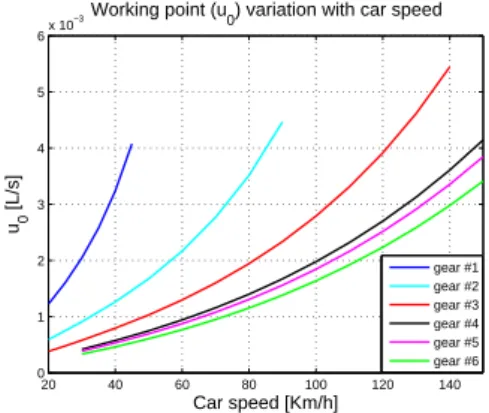
the fuel flow value that allows the car to maintain a station-ary velocity v0. Figure 1 shows the values of u0for a wide

range of stationary velocities, for all the 6 gears. To avoid hybrid dynamics, the actual gear value used is previously selected and held constant throughout the integration of the nonlinear system state equation.

Parameters a and b are chosen to best approximate the nonlinear model response to a step of size δu > 0 (δu small), around the working point (v0, u0), i.e. using a fuel

flow signal u(t) = { u0 t < ts u0+ δu t > ts (5) 20 40 60 80 100 120 140 0 1 2 3 4 5 6x 10

−3Working point (u₀) variation with car speed

Car speed [Km/h] u0 [L/s] gear #1 gear #2 gear #3 gear #4 gear #5 gear #6

Figure 1. Working point fuel flow u0values for all 6 gears

of the nonlinear car model.

where tsis the time instant when the step is applied.

The vehicle velocity evolution resembles the response of a first-order model and, given enough time, it reaches a stationary value after having increased a total of δv. The static gain of the linearized model is thus

K = δv

δu. (6)

The response of the linear model, that corresponds to the integration of (4), is given by

∆v(t) = v0+ δv ( 1− exp ( −t− ts τ )) (7) where τ is the linear system time constant. The value of

τ can be computed either graphically or analytically as the

time instant when the velocity value is ∆v(ts+ τ ) = v0+

δu(1− e−1)≈ v0+ 0.63δu.

Finally, parameter a is the inverse of τ , a = 1

τ, and b

is obtained from K and a as

b = Ka (8)

3 Numerical algorithm for optimal control

Consider the optimal control problem defined in appendix B. The numerical algorithm used to approximate the op-timal control is a gradient based iterative method that pro-ceeds until the stop criterion is met or the maximum num-ber of iterations are reached. Each iteration consists of the following six sequential steps:

1. Integrate state equation

Using the current estimate of the optimal control sig-nal, u(t)∈ Rm, integrate the state equation ˙x = f (x, u, t)

to obtain the state evolution x(t)∈ Rnfrom t0to tf.

2. Integrate co-state equations

Let λΦ(t), an (n×1) vector, and λΨ(t), an (n×q) ma-trix, be co-state variables. Define the corresponding Hamil-tonian functions as

(3)

HΨ(λΨ, x, u, t) = λΨTf (x, u, t),

and integrate backwards, from tf to t0, the co-state

equa-tions −[ ˙λΦ ]T = HxΦ= ∂L ∂x + λ ΦT∂f ∂x, −[ ˙λΨ_]T _{= H}Ψ x = λ ΨT∂f ∂x,

for which the terminal co-state conditions are

λΦ(tf) = ϕTx(x(tf), tf),

λΨ(tf) = ψTx(x(tf), tf).

3. Compute Hamiltonian partial derivatives

Compute the Hamiltonian functions partial deriva-tives in respect to the control signal u for all t∈ [t0, tf],

H_uΦ= ∂L ∂u + λ ΦT∂f ∂u H_uΨ= λΨT∂f ∂u

where HuΦ(t) is a (1× m) vector and HuΨ(t) is a (q× m)

matrix.

4. Compute Lagrange multiplier vector ν Compute ν (a q× 1 vector) by ν =−Q−1g where g = ∫ tf t0 H_uΨ(t)[H_uΦ(t)]Tdt is a (q× 1) vector and Q = ∫ tf t0 H_uΨ(t)[H_uΨ(t)]Tdt is a (q× q) matrix.

5. Compute control correction signal δu(t)

Evaluate ψ at the terminal time and compute the con-trol correction signal δu(t) for all t∈ [t0, tf]

δu(t) =−k[H_uΦ(t) + νTH_uΨ(t)]T− η[H_uΨ(t)]TQ−1ψ(tf)

choosing k < 0 (k > 0) if maximizing (minimizing) the performance index, and 0 < η≤ 1.

Update the estimate of the optimal control signal

u(t)← u(t) + δu(t)

6. Evaluate stop criteria

Compute the root-mean-square value of δu(t)

δurms= 1 tf− t0 ∫ tf t0 [δu(t)]2dt

The algorithm stops if δurms is smaller than a

speci-fied threshold, or if the maximum number of iterations is reached.

4 Minimum energy velocity transfer

The minimum energy velocity transfer (MEVT) consists in transferring the vehicle velocity from a given initial value

v0 at t = t0 to a desired final value vf at t = tf, while

minimizing a quadratic function fuel consumption. This problem may not always be feasible. Depending on the maximum power available for the engine, there is a minimum value of the time interval required to transfer the velocity between two values. This interval depends on the starting velocity as well. Hereafter, we assume that the values specified for the transfer are such that this is feasible. Here, the MEVT problem was considered with t0= 0

and tf = T , for a given value of T , with starting velocity

v(0) = 70 Km/s (u0≈ 1.158 × 10−3L/s) and a given final

velocity v(T ) = vf. The linear model parameters used,

a = 0.04167 and b = 1774.97.

For the linearized model, the performance index for solving the optimal MEVT problem is written as

Jlin(∆u) =− 1 2 ∫ T 0 ∆u(t)2dt (9) in order to minimize the linearized model input: the incre-mental fuel flow ∆u(t). The maximization of this perfor-mance index yields the optimal incremental control signal ∆u∗_lin(t). To obtain the optimal control signal u∗_linwe must add the working point fuel flow value u0, i.e.

u∗_lin(t) = u0+ ∆u∗lin(t) (10)

Thus, in order to allow the comparison between the optimal control signals for both models, nonlinear and linearized, the performance index for solving the optimal MEVT prob-lem using the nonlinear model must also minimize the in-cremental control in respect to u0, i.e.

J (u) =−1 2 ∫ T 0 ( u(t)− u0 )2 dt. (11)

The maximization of this performance index yields the op-timal control signal u∗(t). This is because the linearized problem considers increments with respect to an equilib-rium point, while the nonlinear formulation considers the full range of the variables.

Finally, both u∗_lin(t) and u∗(t) are applied to the non-linear car model, yielding state trajectories v∗_linand v∗, re-spectively. The corresponding cost functional value is also computed in both cases. Notice that using cost functional equation (11) with control signal u∗_lin(t) is the same as us-ing equation (9) with control signal ∆u∗_lin(t).

Results were obtained for some values of terminal time T , which are presented and discussed below.

4.1 Velocity transfer with T = 300 s

With T = 300 s, both systems have enough time to perform the velocity transfer from v0to vf. In fact, careful

(4)

in-0 50 100 150 200 250 300 1.15 1.2 1.25 1.3 1.35 1.4 1.45x 10

−3 Optimal fuel flow

Time [s] Fuel flow [L/s] u*_{(J = −3.3535e−007)} u* lin (J = −3.3086e−007) 0 50 100 150 200 250 300 70 71 72 73 74 75 76

Corresponding car velocity evolution

Time [s] Speed [Km/h] x*_(v f = 75 Km/h) x* lin(vf = 74.9719 Km/h)

Figure 2. Velocity transfer result comparison for T = 300s and vf= 75 Km/h.

terval under consideration the optimal control is fairly con-stant, equal to u0≈ 1.158 × 10−3L/s in order to maintain

the working point speed v0 = 70 Km/h. Furthermore, for

small values of|∆v| = |vf−v0|, the optimal control

devia-tion from the working point fuel flow u0, for which the

lin-earization was designed, is lower and thus u∗_lin(t)≈ u∗(t), naturally yielding x∗_lin(t) ≈ x∗(t). This is the case in fig-ure 2. Figfig-ure 3, where vf = 90 Km/h, shows that values

of vf further away from v0 lead to a higher deviation of

the optimal control in respect to the working point u0, and

thus u∗_lin(t) differs more significantly from u∗(t). In other words, the nonlinear nature of the original model is more noticeable because we are further away from the lineariza-tion working point.

In the particular case of figure 3, the performance in-dex J obtained for optimal control u∗_lin(t) is actually higher than the one obtained for u∗(t), but whereas the achieved final velocity of the latter is v∗(300) ≈ 90.00 Km/h, the former meets the final velocity with much less accuracy,

v_lin∗ (300) ≈ 89.05 Km/h, corresponding to an error . It is then clear that there exists a trade-off between compu-tational effort, which is somewhat lighter when using the linearized model, and the precision in meeting the terminal state restrictions while minimizing fuel flow.

We have seen that for T = 300 s the optimal control sig-nal needs only approximately 150 seconds to increase from

u0to it’s final value (slightly more for vf = 90 m/s), to

meet the terminal velocity constraint. By setting T = 100 s the optimal control magnitude increases slightly, mak-ing it possible to meet the terminal velocity constraint in a smaller time interval.

When vf = 75 Km/h (figure 4) the optimal control

signals are, again, very similar. In fact, when using optimal control u∗_linthe error obtained for the terminal velocity is only 0.0455%. With vf = 90 Km/h (figure 5) the

non-0 50 100 150 200 250 300

1 1.5 2

2.5x 10

Time [s] Fuel flow [L/s] u*_{(J = −5.8139e−006)} u* lin (J = −5.2892e−006) 0 50 100 150 200 250 300 70 75 80 85 90 95

Time [s] Speed [Km/h] x*_(v f = 90.0007 Km/h) x* lin(vf = 89.0511 Km/h)

Figure 3. Velocity transfer result comparison for T = 300 s and vf = 90 Km/h. 0 10 20 30 40 50 60 70 80 90 100 1.15 1.2 1.25 1.3 1.35 1.4 1.45x 10

Time [s] Fuel flow [L/s] u*_{(J = −3.3617e−007)} u* lin (J = −3.3079e−007) 0 10 20 30 40 50 60 70 80 90 100 70 71 72 73 74 75

Figure 4. Velocity transfer result comparison for T = 100 s and vf = 75 Km/h.

linear nature of the original model clearly shows and the resulting optimal control signals are again different. Like before, the performance index is slightly smaller for u∗_lin but the resulting final velocity is also smaller, with an error of 1.075%.

The most noticeable result of reducing the terminal time to

T = 10 s is the increase in the magnitude of the optimal

control signal for both cases, u∗ and u∗_lin. For vf = 75

Km/h (figure 6), both optimal control signals above 1.4× 10−3 L/s whereas before (for T = 300, 100 s) they were below this value. The same happens when vf = 90 Km/h

(figure 7), for which u∗and u∗_linare above 2.2× 10−3L/s whereas before they were mostly below this value.

As a result of the increase in the optimal fuel flow values, which are now further away from the working point fuel flow u0than in the previous cases, the discrepancy

(5)

0 10 20 30 40 50 60 70 80 90 100 1

1.5 2

2.5x 10

Time [s] Fuel flow [L/s] u*_{(J = −5.8533e−006)} u* lin (J = −5.2925e−006) 0 10 20 30 40 50 60 70 80 90 100 70 75 80 85 90

Figure 5. Velocity transfer result comparison for T = 100 s and vf = 90 Km/h. 0 1 2 3 4 5 6 7 8 9 10 1.35 1.4 1.45 1.5 1.55 1.6x 10

Time [s] Fuel flow [L/s] u*_{(J = −5.4914e−007)} u* lin (J = −5.8477e−007) 0 1 2 3 4 5 6 7 8 9 10 70 71 72 73 74 75 76

Figure 6. Velocity transfer result comparison for T = 10 s and vf= 75 Km/h.

the optimal control u∗ provides a better result, achieving the terminal velocity and a performance index that is higher than the one obtained by using the optimal control u∗_lin.

5 Conclusions

For situations that do not require the control signal to de-viate much from the working point fuel flow u0, the

opti-mal control obtained from optimizing the linearized model,

u∗_lin, provides a reasonable, albeit less precise result. If pre-cision is required, it is best to obtain the optimal control by optimizing the original nonlinear model, u∗.

Furthermore, since the fuel flow required to meet the terminal velocity increases when the terminal time T is re-duced beyond a certain threshold, special attention must be given to those situations. It is preferable to use optimal control u∗in those cases.

0 1 2 3 4 5 6 7 8 9 10 2 2.2 2.4 2.6 2.8 3x 10

Time [s] Fuel flow [L/s] u*_{(J = −8.6976e−006)} u* lin (J = −9.3591e−006) 0 1 2 3 4 5 6 7 8 9 10 70 75 80 85 90 95

Time [s] Speed [Km/h] x*_(v f = 89.9999 Km/h) x* lin(vf = 90.6894 Km/h)

Figure 7. Velocity transfer result comparison for T = 10 s and vf= 90 Km/h.

References

[1] Ferreau, H. J., Lorini, G. and Diehl, M. (2006). Fast nonlinear model predictive control of gaso-line engines. Proc. 2006 IEEE Int. Conf. on

Con-trol Applications, Munich, Germany, 2754-2759.

[2] Gausemeir, S., K.-P. Jaker and A. Trachtler (2010). Multi-objective Optimization of a Vehicle Veloc-ity Profile by Means of Dynamic Programming.

Prep. IFAC Symp. Advances in Automotive Con-trol, AAC2010, Munich, Germany.

[3] Hashimoto, S. , Okuda, H., Okada, Y., Adachi, S., Niwa, S. and Kajitani, M. (2006). An engine con-trol systems design for low emission vehicles by generalised predictive control based on identified model. Proc. 2006 IEEE Int. Conf. on Control

Ap-plications, Munich, Germany, 2411-2416.

[4] Kolmanovsky, I. V. and D. P. Filev (2010). Ter-rain and traffic Optimized Vehicle Speed Control.

[5] Luu, H. T., L.Nouvelire and S. Mammar (2010). Dynamic Programming for fuel consumption op-timization on light vehicle. Prep. IFAC Symp.

Ad-vances in Automotive Control, AAC2010, Munich,

Germany.

[6] Saerens, B., J. Vandersteen, T. Persoons, M. Diehl and E. Van den Bulck (2009). Minimization of the fuel consumption of a gasoline engine using dynamic optimization. Applied Energy 86:1582-1588.

[7] T. Jorge, J. M. Lemos and M. Bar˜ao. Optimal cuise control with reduced complexity models.

(6)

[8] Bryson, A. E., and Ho, Y. C. (1975). Applied

Opti-mal Control. Hemisphere, New York.

[9] Bryson, A. E. (1999). Dynamic Optimization. Addison-Wesley.

A

Nonlinear car model equations

1.1 Engine model

The engine model assumes an input diesel flow u(t) mea-sured in liters per second. The total power is given by

P (t) = Eu(t). (12)

where E is the total energy density of diesel fuel and u is the diesel flow. A considerable percentage of this power is dissipated in thermal losses, and only a small part is avail-able as mechanical power, which is thus given given by

Pm(t) = η

(

Te(t), we(t)

)

× P (t). (13)

The engine torque output Teis given by

Te(t) = Pm(t) ωe(t) = η ( Te(t), we(t) ) × P (t) ωe(t) (14) Equation (14) constitutes an algebraic loop, since ef-ficiency η and engine torque values are computed based on each other, which makes computations more taxing. To overcome this, the torque value as a function of we(t) and

u(t) can be numerically computed, by solving the algebraic

loop (14) offline.

For the purposes of this work, it was assumed that efficiency level-curves on the (Te, we) plane are given by

η(Te, we ) = α− β [ (Te− cT)2 lT +(we− cw) 2 lw ] (15) for a reasonable choice of cT, lT, cw and lw. Constants

α and β perform a linear transformation, making the

ellip-tic surface concavity face downwards instead of upwards. Constant α is the value of the maximum efficiency, i.e. when (Te, we) = (cT, cw) then η = α.

In this specific case a closed-form solution for com-puting Te(t) can be easily derived by replacing (15) in (14).

While this is not the general case, it is important to no-tice that a numerical solution with sufficient precision is enough.

From the data available for this engine, it is known that it achieves a maximum torque of 310 Nm at 1800-2400 rpm. Below and above this operational range the torque is greatly reduced. It is also known that a maximum power of 93kW is attained at 3600 rpm, implying a torque T =

93×103 3600

60

2π ≈ 246.7 Nm at that speed.

From this scarce data, a maximum torque curve was designed. For any given engine speed, admissible engine torque values lie below this curve.

1.2 Transmission

The transmission links the wheels and the engine together using a gear box. Its role is to increase torque and decrease wheel speed to match the operational range of the engine. The transmission also introduces internal drag that depends on the engine speed. In the model developed here, the in-ternal drag does not only model the transmission itself, but also all the load at the engine shaft.

The torque output available at the car wheels is given by Tw(t) = rirf ( Te(t)− α − βωe(t) ) (16) where ri is the gear ratio for gear i, rf is the final drive

ratio, α, β are drag coefficients and Te(t), ωe(t) are the

en-gine torque and speed, respectively.

Engine rotational speed, measured in [rad/s], is ob-tained from wheel speed by gear ratio conversion and is given by

ωe(t) = rirfωw(t) (17)

1.3 Traction force and wheels

The wheels are modeled as a rotational to linear move-ment converter neglecting inertia and drag. Wheel rota-tional speed, measured in [rad/s], is given by

ωw(t) =

2π

P v(t) (18)

where P is the wheel perimeter. The used tire dimen-sions are 205/55R16, corresponding to a perimeter of P = 1.9852 meters.

Similarly, traction force is obtained from the torque applied by the engine at the wheels

F (t) = 2π

P Tw(t) (19)

B

Iterative numeric solution of the optimal

control problem with terminal constraints

Using the methods of [8, 9], this appendix shows how to construct a history δu(t) that optimizes the performance index by making the control signal converge to the opti-mal control u∗(t). To simplify the notation, we shall make

∂f ∂x ≡ fx, ∂f ∂u ≡ fu, ∂L ∂x ≡ Lxand ∂L ∂u ≡ Lu. Let ˙ x = f (x, u, t), t∈ [t0, tf] (20)

describe the generally nonlinear time-varying dynamics of a plant, where x(t) ∈ Rn _{and u(t)} _{∈ R}m_{are the}

state-vector and input state-vector at time t, respectively, and

J = ϕ(x(tf), tf) +

∫ tf

t0

L(x(t), u(t), t)dt (21)

a performance index, associated with the above plant, which we wish to maximize. A minimization problem

(7)

can also be formulated by maximizing the performance index Jmin = −J. Notice that function ϕ(x(tf), tf) is

a function of the terminal state and terminal time, while

L(x(t), u(t), t) depends on the state, input and time values

in the interval [t0, tf].

The optimal control problem consists in finding input signal u∗(t), t ∈ [t0, tf], for which the plant exhibits a

state trajectory x∗(t), such that the cost functional value,

J , is maximum. Additionally, one might wish to introduce

restrictions on the terminal state value, in the form of q restriction equations ψ(x(tf), tf) =  ψ1(x(t_{· · ·}f), tf) ψq(x(tf), tf)   =  _{· · ·}0 0   . (22)

The problem is thus to maximize the performance index (21) subject to constraints (20) and (22).

As is well known, the solution to this problem satis-fies the set of necessary conditions:

1. State equation Hλ− ˙xT = 0⇔ ˙x = HλT = f (x(t), u(t), t), (23) 2. Co-state equation Hx+ ˙λT = 0⇔ − ˙λT = Hx= ∂L ∂x + λ T∂f ∂x, (24)

3. Final state condition

ψ(x(tf), tf) = 0, (25) 4. Stationarity condition Hu= 0⇔ ∂H ∂u = ∂L ∂u + λ T∂f ∂u, (26) 5. Boundary condition [(ϕx+ νTψx− λT)dx]t=tf = 0, (27)

Assume now that we wish to constrain the ith com-ponent of the state vector by prescribing a fixed value at the terminal time, xi(tf). It follows that dxi(tf) = 0 and

thus in order to satisfy the boundary equation (27) it is not necessary that [_∂x∂ϕ

i − λ

T

i]t=tf = 0. In fact, we have

sim-ply traded this latter boundary condition for another one, namely xi(tf) given. If we wish to prescribe a fixed value

at the terminal time for first q components of the state vec-tor, then

δxi(tf) = 0, i = 1, ..., q (28)

and thus ϕ is a function of the remaining components of the state vector

ϕ = ϕ(xq+1, ..., xn)t=tf. (29)

It is more general to prescribe a fixed value for the terminal state by means of a function written in the format

ψi(xi(tf), tf) = 0, i = 1, ..., q. (30)

for which, if the terminal time tfis fixed, we can derive the

following relation

δψi(xi(tf), tf) = 0⇔ δxi(tf) = 0 (31)

Henceforth we shall use ψi(tf) ≡ ψi(xi(tf), tf) to

sim-plify notation. We derive now an equation for the variation of the augmented performance

d ¯J = [(ϕx− λΦT)dx]t=tf+ + ∫ tf t0 [(H_xΦ+ [ ˙λΦ]T)δx + H_uΦδu + (H_λΦΦ− ˙x T_)δλΦ_]dt, (32) where the superscript Φ is used to differentiate from analo-gous variables introduced later.

Knowing that the first q components of the state vec-tor are prescribed at the terminal time

ψ(x(tf), tf) =      ψ1(tf) ψ2(tf) .. . ψq(tf)     =      0 0 .. . 0     , (33)

by replacing equations (23), (24) and (27) into (32) it fol-lows that d ¯J = ∫ tf t0 [H_uΦδu]dt = ∫ tf t0 [( Lu+ λΦTfu ) δu ] dt (34) where HΦ= L + λΦTf, (35) −[ ˙λΦ_]T _{= H}Φ x = Lx+ λΦTfx, (36) λΦi(tf) =    0, i = 1, ..., q ( ∂ϕ ∂xi ) tf , i = q + 1, ..., n (37)

Assume that, instead of (21), the performance index was

J′ = ψi(xi(tf), tf), i.e. the function that prescribes

the ith component of the state vector at the terminal time. This corresponds to making the objective func-tion ϕ′(x(tf), tf) = ψi(tf) and the lagrangian function

L′(x, u, t) = 0. Then the equivalent expressions to (34), (36), and (37) can be written as

d ¯J′= δψi(tf) = ∫ tf t0 [H_u(i)δu]dt = ∫ tf t0 [( λ(i)Tfu ) δu ] dt (38) where H(i)= λ(i)Tf, (39) −[ ˙λ(i)_]T _{= H}(i) x = λ(i)Tfx, (40)

(8)

λ(i)_k (tf) =    0, k̸= i ( ∂ψi ∂xi ) tf , k = i k = 1, ..., n (41)

We shall now construct a history δu(t) that increases J

(d ¯J > 0) and satisfies the q terminal constraints (30).

Mul-tiply each of the q equations (38) by an undetermined con-stant νi, and add the resulting equations to (34)

d ¯J + q ∑ i=1 {νiδψi(tf)} = d ¯J + νTδψ(tf) ∫ tf t0 ( Lu+ [ λΦ+ λq]Tfu ) δudt (42) where ν =[ν1 ν2 · · · νq ]T , (43) λq= q ∑ i=1 { νiλ(i) } , (44)

and ψ(tf) ≡ ψ(x(tf), tf) to simplify notation. Now,

choose δu=−k ( fuT [ λΦ+ λq]+ LTu ) (45) where k is a negative scalar constant, and substitute this expression into (42), as follows

d ¯J + νTδψ(tf) = −k ∫ tf t0 fuT[λ Φ + λq] + LTu 2 dt, (46)

that is always positive unless the integrand vanishes over the whole integration interval. Next we determine the value of constants νi in order to satisfy the terminal constraints

(30). Substituting (45) into (38), we have 0 = δψi(tf)⇔ ⇔ 0 = −k ∫ tf t0 λ(i)Tfu ( f_uT[λΦ+ λq] + LT_u)dt ⇔ 0 = ∫ tf t0 λ(i)Tfu [ f_uTλΦ+ LT_u]dt+ ∫ tf t0 λ(i)TfufuTλ q_dt ⇔ 0 = ∫ tf t0 λ(i)Tfu [ f_uTλΦ+ LT_u]dt+ + q ∑ j=1 { νj ∫ tf t0 λ(i)TfufuTλ (j)_dt } ⇔ 0 = gi+ q ∑ j=1 {νjQij} (47) where gi= ∫ tf t0 λ(i)Tfu [ f_uTλΦ+ LT_u]dt = ∫ tf t0 H_u(i)[H_uΦ]Tdt, (48) Qij = ∫ tf t0 λ(i)TfufuTλ (j)_{dt =} ∫ tf t0 H_u(i)[H_u(j)]Tdt. (49)

The q equations (47) can be written in matrix format as 0 = g + Qν

where Q is the (q×q) terminal state controllability matrix. By defining

λΨ=[λ(1) _λ(2) _{· · · λ}(q)] ₍₅₀₎

an (n× q) matrix and

HΨ=[H(1) _H(2) _{· · · H}(q)]T _{= λ}ΨT_f, ₍₅₁₎

a q-component column array, one can also write

g = ∫ tf t0 HuΨ[HuΦ]Tdt, (52) Q = ∫ tf t0 H_uΨ[H_uΨ]Tdt. (53)

The appropriate choice for the multipliers νjis then

ν =−Q−1g. (54)

If Q is a singular matrix, Q−1does not exist, meaning that it is not possible to control the system with u(t) in order to satisfy one or more of the terminal conditions.

We have thus constructed a δu(t) history that in-creases the performance index and satisfies the terminal constraints (30). From (46) the only case in which we can-not increase the performance index is when

Lu+ [λΦ+ λq]Tfu= 0, t0≤ t ≤ tf (55)

If (55) is satisfied, we have a stationary solution that satisfies the terminal constraints.