Lat. Am. j. solids struct. vol.11 número14

(1)

Abstract

In this paper, the global optimal path planning of an autonomous vehicle for overtaking a moving obstacle is proposed. In this study, the autonomous vehicle overtakes a moving vehicle by performing a double lane-change maneuver after detecting it in a proper dis-tance ahead. The optimal path of vehicle for performing the lane-change maneuver is generated by a path planning program in which the sum of lateral deviation of the vehicle from a reference path and the rate of steering angle become minimum while the lateral acceleration of vehicle does not exceed a safe limit value. A nonlinear optimal control theory with the lateral vehicle dynamics equations and inequality constraint of lateral acceleration are used to generate the path. The indirect approach for solving the opti-mal control problem is used by applying the calculus of variation and the Pontryagin’s Minimum Principle to obtain first-order necessary conditions for optimality. The optimal path is generated as a global optimal solution and can be used as the benchmark of the path generated by the local motion planning of autonomous vehicles. A full nonlinear vehicle model in CarSim software is used for path following simulation by importing path data from the MATLAB code. The simulation results show that the generated path for the autonomous vehicle satisfies all vehicle dynamics constraints and hence is a suitable overtaking path for the follow-ing vehicle.

Keywords

Path planning; autonomous vehicle; optimal control; Pontryagin’s minimum.

Global optimal path planning of an autonomous vehicle for

overtaking a moving obstacle

Notations ob

a obstacle longitudinal acceleration (m/s2) y

a vehicle lateral acceleration (m/s2) C_a tire cornering stiffnesses (N/rad)

y

F lateral tire force (N)

B. Mashadia M. Majidib

School of Automotive Engineering, Iran University of Science and Technology

Corresponding autor: a_{b_mashhadi@iust.ac.ir} b_{m_majidi@iust.ac.ir}

(2)

Latin American Journal of Solids and Structures 11 (2014) 2555-2572

g acceleration due to gravity (m/s2) z

I vehicle moment of inertia about the yaw axis (kg m2) f

l distance from the vehicle CG to the front axle (m)

r

l distance from the vehicle CG to the rear axle (m)

m vehicle mass (kg)

u control input

U vehicle longitudinal speed (m/s)

0

ob

U obstacle initial speed (m/s) v vehicle lateral speed (m/s)

x state vector

x vehicle displacement along the reference path (m) y lateral deviation of vehicle from the reference path (m) a tire slip angle (rad)

f

d steering angle of the front wheels (rad) y heading angle (rad)

Subscripts

f front

l left

1 INTRODUCTION

There is a recent trend in the automobile industry towards autonomous vehicles. The autonomous vehicle, also known as driverless vehicle is a kind of vehicle capable of sensing its environment and navigating along a predefined path without driver intervention. Motion planning is one of the im-portant aspects of an autonomous vehicle motion. It deals with the search and execution of colli-sion-free paths by performing specific tasks. Motion planning consists of two stages, path planning and path tracking. The path planning stage involves the search and computation of a collision-free path, taking into account the geometry of vehicle , its surroundings and obstacles, the vehicle kin-ematic constraints, and sometimes dynamics constraints as well as any other external constraints that may affect the planning of a path (Park et al., 2009). The path tracking stage involves the actual navigation on the planned path considering the kinematic and dynamic constraints of the vehicle (Kim et al., 2011; Mashadi et al., 2014).

(3)

researches (Purwin and D’Andrea, 2006; Park et al., 2009; Yoon et al., 2009; Zhe et al., 2009; Matveev et al., 2011).

There are two optimization approaches which are used for path panning of autonomous vehicles. The local optimal path planning, which needs to predict the future of the system, is used in real time vehicle obstacle avoidance systems. The main objective of obstacle avoidance systems is to avoid obstacles based on the data collected from the onboard sensors. It may be used when the vehicle encounters an unexpected obstacle during following a pre-computed path. Since local path planners run in real time and on onboard computers that usually have very limited computing ca-pabilities, they have to be efficient in terms of both memory utilization and time. Most of the re-searches on the local obstacle avoidance have been performed using reactive methods based on the sensor data (Spenko et al., 2004; Minguez and Montano, 2005; Garg et al., 2011). Some researches take into account the simple robot dynamics in terms of velocity or turning radius (Yuan et al., 2006). These approaches are computationally efficient, but the vehicle can get stuck in local mini-ma. Some recent researches are accomplished by using advanced algorithms such as Model Predic-tive Control (MPC) (Borrelli et al., 2005; Park et al., 2009; Yoon et al., 2009; Nanao and Ohtsuka 2010) or Fuzzy Logic (Naranjo et al., 2008). Their efficiency is usually measured by the amount of time they take. The quality of their results depends on the amount of look-ahead distance of the sensors (Isermann et al., 2008).

On the other hand, the main objective of global optimal path planning is to determine appropri-ate control laws for steering an autonomous vehicle between two pre-described points in the stappropri-ate space. The autonomous vehicle uses the path information to navigate itself efficiently through the environment with the help of a path tracking algorithm. Some approaches have been explored for obtaining the optimal path using search methods such as Genetic Algorithms (GA) (Onieva et al., 2011) or computational methods such as optimal control. Thus, the produced path of the global optimal path planning can be used as a benchmark for the path generated by the local motion planning of the autonomous vehicle. Therefore, designing an autonomous vehicle, consisting of an individual one or a group of cooperating vehicles, is possible when motion planning of vehicles can be done. Thus, path planning is the most fundamental issue for designing an autonomous vehicle. In this paper, an efficient global path planning algorithm that is capable of finding optimal colli-sion-free paths from a start point to a goal is developed. The Pontryagin’s Minimum Principle (PMP) is used to solve the optimal control problem for obtaining the optimal path planning. The paper is structured as follows. Section 2 describes path planning program which is used to generate optimal trajectories for the vehicle. Section 3 discusses the simulation results. Conclusions are pre-sented in section 4.

2 MODELING OF PATH PLANNING PROGRAM

(4)

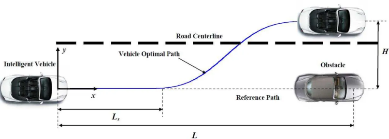
path planning program. Due to the probability of frontal crash in the opposite lane, the autono-mous vehicle should move close to the obstacle as much as possible to minimize the sum of lateral deviation of the vehicle relative to the previous path. On the other hand, if the vehicle closes too much to the obstacle, vehicle lateral acceleration during the lane-change maneuver becomes too high. Since in high lateral acceleration maneuvers, autonomous vehicle might become unstable, the path should be obtained such that the vehicle lateral acceleration during the lane-change maneuver does not exceed a safe limit.

Figure 1: Schematic diagram of the lane-change maneuver.

Since the optimality of path is global the start and end points of vehicle travel during the ma-neuver are known; so, to define the cost function of the optimal problem, it is assumed that the autonomous vehicle detects the obstacle at distance L₀ in front of itself and after traveling a

dis-tance L along the reference path, the vehicle succeeds to complete the lane-change maneuver and

overtake the obstacle. As shown in Figure 1, the autonomous vehicle first travels a distance L_s

along the reference path and then executes the lane-change maneuver in such way that the vehicle final lateral deviation from the reference path becomes H and the lateral acceleration of vehicle

doesn’t exceed a predefined safe limit. The path is obtained in the inertial reference frame which is coincident on the vehicle reference frame at the moment of decision making for the lane-change maneuver. The origin of vehicle reference frame is located at the center of vehicle front axle. So the cost function of the path planning program is defined as:

(

2 2

)

1 2 ₀

f

t

f

J =

ò

y +wd dt (1)

where y is the vehicle path deviation from the reference path, d_f is the rate of front wheel steering

angle and w is a weighting factor that indicates the relative importance of the corresponding term.

(5)

2.1 Vehicle dynamics modeling

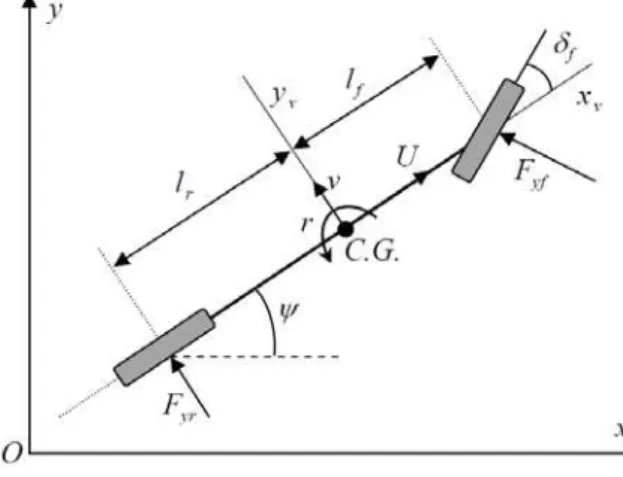
A simplified linear bicycle model (see Figure 2) is used to determine the optimal path. The vehicle degrees of freedom are lateral velocity in direction y_v and the yaw rate around the z axis.

Govern-ing equations of the bicycle model can be described as follows(Mashadi et al., 2014):

Figure 2: 2-DOF vehicle dynamics model.

2 2

f r f f r r f

f

f f r r f f r r f f

f

z z z

C C l C l C C

v v U r

mU mU m

l C l C l C l C l C

r v r

I U I U I

r

a a a a a

d

y

ì æ + ö æ - ö æ ö

ï _ç _÷ _ç _÷ _ç _÷

ï = -_ç ÷ + -_ç - ÷ +_ç ÷

ï _ç_ç ÷_÷ _ç_ç ÷_÷ _ç_ç ÷_÷

ï è ø è ø è ø

ïïï æ _- ö æ ₊ ö_÷ æ ö

í çç ÷÷ çç ÷ ç ÷÷

ï = -ç ÷ + -ç ÷ +ç ÷

ï ç ÷ ç ÷ ç ÷

ï çè ÷ø ç ÷÷ ççè ÷ø

ï è ø

ïï ï = ïî



(2)

where U and v stand for the longitudinal and lateral velocities of vehicle center of gravity (CG),

respectively. m is the vehicle mass, I_z is the yaw moment of inertia, r and y are the vehicle yaw

rate and yaw angle, respectively; lf and lr are the distances from vehicle CG to the front and rear

axles. Caf and Car denote the cornering stiffnesses of the front and rear tires, respectively.

The vehicle motion in the inertial reference frame is described by:

(

)

(

)

cos sin

f

x U v l r

y v l r U

y y

ìï = - +

ïí

ï = + +

ïî



 (3)

where x is the vehicle displacement along the reference path. Although the actual input command

to the vehicle dynamics is the steering angle of the front wheels, d_f , the input is redefined to be d_f , and df is set to be a state variable of the system so that the rate of change of df can be

con-strained by placing a limit on the system input u. Setting the state vector as T

f

v r y x y d

é ù

= ê_ë ú_û

(6)

( ) u

= +

x f x B (4)

where,

(

)

(

)

2 2 ( ) cos sin cos si

f r f f r r f

f

f f r r f f r r f f

f

z z z

f

C C l C l C C

v U r

mU mU m

l C l C l C l C l C

v r

I U I U I

r

U v l r

v l r U

a a a a a

d

y y

y

æ + ö_÷ æ - ö_÷ æ ö_÷

ç _÷ ç _÷ ç _÷

ç- ÷ + -ç - ÷ +ç ÷

ç ÷ ç ÷ ç ÷

ç ç ç

è ø è ø è ø

æ ö

æ - ö_÷ _ç + _÷ æ ö_÷

ç ÷ ç ÷ ç ÷

ç- ÷ + -ç ÷ +ç ÷

ç ÷ ç ÷ ç ÷

ç ÷ ÷ çç ÷

ç ç ÷ è ø

è ø è ø

= - + + + f x n 0 y é ù ê ú ê ú ê ú ê ú ê ú ê ú ê ú ê ú ê ú ê ú ê ú ê ú ê ú ê ú ê ú ê ú ë û 0 0 0 0 0 1 é ù ê ú ê ú ê ú ê ú ê ú = ê ú ê ú ê ú ê ú ê ú ê ú ë û

B u =df

It should be noted that although the vehicle dynamics equation (2) is linear, the state equation (4) is nonlinear due to the presence of nonlinear terms in equation (3), and hence the optimal problem is also nonlinear.

To ensure that the actual vehicle can track the generated path based on this simplified model, the assumptions placed on the vehicle model should be satisfied. The assumptions made during deriving this model imply that the tire lateral force versus tire slip angle is bounded in the linear regime. This leads to a direct constraint on the slip angles to have small values. If the constraints on the tire slip angles were to be used, complicated derivative terms would appear in the nonlinear optimization process. Instead of two individual constraints, the following constraint on the lateral acceleration is used, because it has the same effect on keeping the values of tire slip angles small.

y yc

a = v+Ur £a (5)

where ay is the lateral acceleration of the vehicle and ayc is the maximum value of vehicle lateral

acceleration in which the lateral tire forces are bounded in the linear regime. The desired value of

yc

a is evaluated in the simulation section. By substituting v from equation (2) into (5) and

intro-ducing functionC( )x , the lateral acceleration constraint is written as:

( ) C f C r l Cf f l Cr r C f _f _yc 0

C v r a

mU mU m

a a a a a _d

æ + ö_÷ æ - ö_÷ æ ö_÷

ç _÷ ç _÷ ç _÷

ç ç ç

= -_ç_ç _÷÷_÷ + -_ç_ç _÷÷_÷ +_ç_ç _÷÷_÷ - £

ç ç ç

è ø è ø è ø

x (6)

in which ayc is a given limit of the lateral acceleration. The optimal path for the autonomous

vehi-cle should be obtained in such way that the input control of vehivehi-cle during tracking does not exceed the saturation limit. Since the control input of vehicle is defined as the steering angle rate, the satu-ration limit of the control input depends on the steering mechanism of the vehicle presented as:

sat

u £u (7)

(7)

2.2 Optimal Path planning problem

For obtaining the optimal path, the cost function (1) is to be solved together with the vehicle dy-namics constraint (4), the lateral acceleration constraint (6), and control input constraint (7). The Pontryagin’s Minimum Principle is used for solving the nonlinear optimal control problem. First, cost function (1) is rewritten as:

(

2 2

)

(

2

)

1 1 1

2 0 0 2 2

f f

t t

T f

J =

ò

y +wd dt =

ò

x Qx + wu dt (8)

where Q denotes positive weighting matrices. Since the vehicle path is straight in the beginning of the time interval and the end of the lane-change maneuver is also straight, the state variables in-cluding lateral velocity, yaw rate, heading angle and steering angle of vehicle in the beginning and end of the time interval become zero. So, boundary conditions of the vehicle are defined as follows:

(0)= ( )t_f = êé_ë0 0 0 L H 0ù_ú_ûT

x 0 x (9)

The final time tf , is free and should be obtained by solving the optimal control problem. If the

obstacle is moving with a constant deceleration a_ob, the final distance along the reference path is

calculated from:

2 1

0 0 2

( )_f _ob _f _{ob f}

x t =L =L +U t + a t (10)

where U_ob₀ is initial speed of the obstacle at the moment of decision making for the lane-change

maneuver. The Hamiltonian is defined as (Kirk 2004):

(

)

2 2

1 2

( ( ), ( ), ( )) T T ( ) ( )Heaviside( ( ))

c

t t u t = 1 w u +1w C C

2 2

x P x Qx + + P f x + Bu x x

H

(11)

where P is the Lagrange multiplier vector for the vehicle dynamics constraint, and w_c is the

weighting parameter for the inequality constraints on the lateral acceleration. The Heaviside func-tion is defined as:

1 ( ) 0

Heaviside( ( ))

0 ( ) 0

C C

C ì > ïï

= í_ï _£

ïî

x x

x

The co-state equations can be presented in the following form:

( ) ( )

( )T Heaviside( ( ))

c C

w C

¶ ¶

¶

= - = - -

-¶ ¶ ¶

f x x

P Qx P x

x x x

H

 ₍₁₂₎

In order that _u*_{be an optimal solution of equation (1), the following is a necessary condition (Kirk}

(8)

* _{arg min( ( , , ))} _{[0, ]}

f

u =

H

x Pu " Ît t (13)

In the case that the control input value is smaller than the saturation limit defined in the inequality constraint (7), the first derivative of

H

with respect to u is equal to zero, so:

* * * 1

( , ,u ) w u T 0 u w T

u

-¶ ₌ ₊ ₌ _ ₌

-¶ x P B P B P

H

₍₁₄₎

To insure that the Hamiltonian at the derived control input is minimum, the second derivative test is applied:

2

2 w 0

u

¶ ₌ _> ¶

H

₍₁₅₎

As the second derivative of the Hamiltonian with respect to u is positive, the control input

ob-tained by equation (14) is the minimum point of Hamiltonian and it becomes the solution of the optimal control problem. In the case that the control input is greater than the saturation limit, the control input that minimizes the Hamiltonian is equal to the saturation limit. By Substituting B

from equation (4) in (14) and considering what mentioned before, the optimal control input is ob-tained as:

* 1

6 6

*

6

( ) ( )

sgn( ( ))

sat

if P t w u then u w P t

else u P t u

-ìï £ =

-ïïí

ï =

-ïïî (16)

where P t₆( ) is the sixth element of the co-state vector and sgn is the sign function. By applying the

calculus of variation method to the cost function subject to the constraint, the following boundary condition between the final state and co-state variables is presented as:

(

_{( ), ( ),} *_{( )}

)

_{( )}T ₀

f f f f f

t t t dt - t d _f =

x P u P x

H

(17)

All of final states are specified expect the distance along the reference path x t( )f , so by taking the

variation from equation (10), the variation of final unspecified state is derived as:

(

0

)

f ob ob f f

x U a t t

d = + d (18)

By substituting the equation (18) into (17), the following equation is obtained:

(

)

(

)

(

*

)

0 4

( ), ( ),t_f t_f ( )t_f - U_ob +a t_{ob f} P t( )_f dt_f =0

x P u

H

(19)

Because the final time tf is free in this optimal control problem, its variation, dtf, is nonzero and

(9)

(

*

)

(

)

0 4

( ), ( ),t_f t_f ( )t_f - U_ob +a t_{ob f} P t( )_f =0

x P u

H

(20)

The Hamiltonian function at the final time is calculated by replacing the time with tf and

substi-tuting equations (9) and (14) into (11) as the following statement:

(

*

)

1 2 1 1 2

6 4

2 2

( ), ( ),t_f t_f ( )t_f = H - w- P ( )t_f UP t( )_f

x P u +

H

(21)

Then, by substituting the equation (21) into (20), the following boundary condition in the final time is obtained:

(

)

2 1 2

0 4 6

2 _ob _{ob f} ( )_f ( )_f 0

H + U -U -a t P t -w-P t = (22)

By using differential equations (4), (12), control input (16) and boundary conditions (9) and (22), the two point boundary value nonlinear optimal control problem is presented as:

(

)

* * 1 6 6 * 6 2 1

0 0 ₂

2 1 2

0 4 6

( ) ( )

( ) Heaviside( ( ))

( ) ( )

sgn( ( ))

(0)

( ) 0 0 0 0

2 ( ) ( )

T c

sat

T

f ob f ob f

ob ob f f f

u

C

w C

if P t w u then u w P t

else u P t u

t L U t a t H

H U U a t P t w P t

-ìï = + ïïï

í ¶ ¶

ï = - -

-ïïïî ¶ ¶

ìï £ =

-ïïí

ï =

-ïïî =

é ù

= _ê_ë + + _ú_û

- -

-x f(x) B

f x x

P Qx P x

x x x 0 x +   0 ìïï ïï ïï íï ïï ï ₌ ïïî (23)

For solving the above two point boundary value problem, the “bvp5c” function in MATLAB soft-ware is used (Wang, 2009). Since the time interval should be fixed in the function, the independent variable tcan be changed to t =t tf in equation (23) as:

(

)

(

)

* * 1 6 6 * 6 2 1

0 0 ₂

2

( ) ( ) ( )

( )

( ) ( ) ( ) ( ) Heaviside ( )

( ) ( )

sgn( ( ))

(0)

(1) 0 0 0 0

f T f c sat sat T

ob f ob f

t u

C

t w C

if P w u then u w P

else u P u

L U t a t H

H

t t t

t t

t

-ìï = +

ïïï _æ _ö

í _ç ¶ ¶ _÷

ï = ç- - - ÷

ï _ç_ç ÷_÷

ï _è _¶ _¶ _ø

ïî

ìï £ =

-ïïí

ï =

-ïïî =

é ù

= _ê_ë + + _ú_û

x f(x ) B

f(x) x

P Qx P x

x x

x 0

x  

(

)

1 2

0 4 6

2 U U_ob a t_{ob f} P(1) w-P (1) 0

ìïï ïï ïï íï ïï

ï _- _- _- ₌

ïïî +

(10)

Now the problem is set on the fixed interval [0 , 1]. By solving the boundary value problem (24) in MATLAB and calculating the state variables in the time interval [0 ,t_f], optimal path of the

au-tonomous vehicle for overtaking the moving obstacle is obtained.

3 SIMULATION RESULTS

In this section, the numerical solutions of the boundary value problem for planning the optimal path and the simulation of the vehicle dynamics response during tracking the generated path are presented. In simulations throughout the paper, the path generated by the path planning programs is applied to the CarSim vehicle model. CarSim is a software which builds full nonlinear models of actual vehicles when parameters such as dimensions of the vehicle platform, specifications of the engine and tires, and coefficients of the suspensions are given. The CarSim vehicle model has been validated with experimental results of an actual vehicle (Yoon et al., 2009). The parameters charac-terizing a typical vehicle used for path planning are given in Table 1. Two simulations are prepared in this section. In the first simulation, the autonomous vehicle and the obstacle are moving on a straight road but in the second one, they are moving on a circular road. For every simulation, the boundary value problem equation (24) should be solved first with proper lateral acceleration con-straint, and then the generated path is imported to CarSim for path tracking simulations to demon-strate the suitability of the generated path.

Parameter Value Parameter Value

m(kg) 1300 I_z(kg m2) 2500 f

l (kg) 1.2 Caf (N m s/ rad) 80800

r

l (m) 1.3 Car (N m s/ rad) 76100

Table 1: Vehicle Parameters for the path planning program.

For solving the optimal path planning problem presented in equation (24), the acceleration ayc

of the autonomous vehicle must be evaluated. To determine a reasonable value for a_yc, the bicycle

model is compared with the CarSim model in the Simulink environment. By applying an exponen-tially increasing sinusoidal steering maneuver shown in Figure 3(a) to both models, performed at 100 km/h, a comparison between the bicycle model and the CarSim model is represented in Figure 3.

As illustrated in Figures 3(b) and 3(c), the lateral velocity and yaw rate of the two models agree with each other when the magnitude of the lateral acceleration shown in Figure 3(e) is under 0.3g. For the values of lateral acceleration exceeding 0.3g after 2.5 sec, the lateral velocity and yaw rate of the two models start to deviate. This is due to significantly large tire slip angle generation shown in Figure 3(d). Because of using the linear lateral tire model which is valid in the range of

2 a 2

-  £ £ _{for the bicycle model, the lateral tire forces of the two models start to differ from}

(11)

each other. So, the desired value of lateral acceleration ayc for the inequality constraint of boundary

value problem (24) is chosen as 0.3g.

(a)

(b) (c)

(d) (e)

Figure 3: Comparison between the bicycle model and CarSim vehicle model: a) front wheel steering applied to the

CarSim and bicycle model (deg), b) lateral velocity (m/s), c) yaw rate (deg/s), d) front tire slip angle (deg) e) lateral acceleration (g) of the CarSim model and bicycle model.

3.1 Obstacle moving on a straight path

For solving the optimal path planning problem in the first simulation, the vehicle and the obstacle speeds are considered constant as 30 m/s and 10 m/s, respectively. The initial distance between the

0 1 2 3 4 5 6

-6 -4 -2 0 2 4 6 Time (sec) Fr ont whe e l s teer in g a ngl e ( d e g )

0 1 2 3 4 5 6

-2.5 -2 -1.5 -1 -0.5 0 0.5 1 1.5 2 2.5 Time (sec) Lat er al vel o c ity ( m /s ) CarSim model Bicycle model

0 1 2 3 4 5 6

-40 -30 -20 -10 0 10 20 30 40 Time (sec) Y a w ra te (d e g /s ) CarSim model Bicycle model

0 1 2 3 4 5 6

-4 -3 -2 -1 0 1 2 3 4 Time (sec) Fr ont t ir e sl ip angl e ( deg /s ) CarSim model Bicycle model

0 1 2 3 4 5 6

(12)

vehicle and the obstacle on the straight road is considered as 200 m. By numerically solving the two point boundary value problem (24) with the lateral acceleration constraint of 0.3g, the optimal state variables and control input are obtained and shown in Figure 4.

(a) (b)

(c) (d)

Figure 4: Path planning results: a) optimal path of vehicle, b) heading angle (deg), c) steering angle (deg), d)

lat-eral acceleration (g) of vehicle for performing the lane-change maneuver on straight road.

Figure 4(a) shows the lateral deviation from the reference path (y) versus the distance along the

reference path (x). Since the reference path is straight, the plot of variable y versus x implies the

path of vehicle in the global coordinate during the overtaking maneuver. The autonomous vehicle first moves forward about 210 m along the reference path and then carries out a lane-change ma-neuver to change its lane of motion to overtake the moving obstacle.

Figure 4(b) shows the heading angle of vehicle during the maneuver. As it can be seen, the vehi-cle execute the maneuver with small heading angle which this demonstrate the vehivehi-cle stability during the maneuver. The vehicle steering angle is shown in Figure 4(c). Figure 4(d) demonstrates lateral acceleration of the autonomous vehicle for performing the lane-change maneuver. It can be seen that the value of the lateral acceleration does not exceed 0.3g as expected. Also, it is illustrated that the autonomous vehicle deviates to right about 0.3 m just before turning to the left to accom-plish the lane-change maneuver. This is due to discontinuity of the control input at the start point

0 50 100 150 200 250 300

-0.5 0 0.5 1 1.5 2 2.5 3

x (m)

y (

m

)

0 2 4 6 8 10

-1 0 1 2 3 4 5 6

Time (sec)

H

eadi

ng angl

e (

deg)

0 2 4 6 8 10

-0.8 -0.6 -0.4 -0.2 0 0.2 0.4 0.6

Time (sec)

St

eer

ing angl

e (

deg)

0 2 4 6 8 10

-0.4 -0.3 -0.2 -0.1 0 0.1 0.2 0.3

Time (sec)

Lat

er

al

ac

cel

e

ra

tion (

g

(13)

of the lane-change section of the path. To resolve this unexpected deviation in the vehicle path, it is needed to define two cost functions. One for the straight section and the other for the lane-change section of the path. The optimal path generated by defining two phase cost function is focused in our further research.

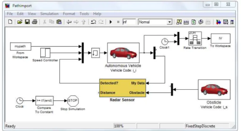
By importing the CarSim model to the Simulink environment, the path generated by the path planning program is tracked by an autonomous vehicle built in the CarSim. As shown in Figure 5, the autonomous vehicle and the obstacle vehicle model built in the CarSim are connected together through Simulink Environment. For overtaking the obstacle, the autonomous vehicle should per-form a double lane-change maneuver. Since the generated path represented in Figure 4(a) is a single lane-change maneuver, the path planning program should combine two generated paths symmetri-cally with respect to the obstacle for obtaining the path of a double lane-change maneuver. Figure 6(a) shows the optimal path generated by the path planning program and the path tracked by the vehicle. It shows that the vehicle can track the generated path precisely. Figure 6(b) demonstrates the front wheel steering angle during the double lane-change maneuver. As shown in Figure 6(b), the actual steering angle extrema are similar to what obtained by the path planning problem. Fig-ure 6(c) also shows the actual lateral acceleration of vehicle tracking the generated path. It can be seen that the value of vehicle lateral acceleration is always smaller than 0.3g. So, the autonomous vehicle is tracking the generated path as its dynamic response is equal to the original bicycle model for which the optimal path is generated.

Figure 5: The CarSim vehicle model simulated in the Simulink environment.

3.2 Obstacle moving on a straight path with deceleration

(14)

acceleration of vehicle is shown in Figure 7(b). Like the first simulation, the vehicle performs the lane-change maneuver with lateral acceleration bounded below the 0.3g.

(a)

(b) (c)

Figure 6: Path tracking results from the CarSim: a) optimal and actual paths, b) actual steering angle (deg), c)

actual lateral acceleration (g) of vehicle during double lane-change maneuver in the straight road.

(a) (b)

Figure 7: Path planning results: a) optimal path, b) lateral acceleration of vehicle (g) for overtaking the obstacle

with deceleration.

0 100 200 300 400 500 600

-0.5 0 0.5 1 1.5 2 2.5 3 3.5

Global x coordinate (m)

G

lobal

y

c

oor

di

nat

e (

m

)

Optimal path Vehicle path

0 2 4 6 8 10 12 14 16 18 20

-1 -0.8 -0.6 -0.4 -0.2 0 0.2 0.4 0.6 0.8 1

Time (sec)

S

teer

ing angl

e(

deg)

0 2 4 6 8 10 12 14 16 18 20

-0.4 -0.3 -0.2 -0.1 0 0.1 0.2 0.3

Time (sec)

Lat

er

al

ac

ce

le

ra

ti

o

n

(g

)

0 50 100 150 200 250

-0.5 0 0.5 1 1.5 2 2.5 3

X(m)

Y(

m)

0 1 2 3 4 5 6 7 8

-0.4 -0.3 -0.2 -0.1 0 0.1 0.2 0.3

Time (sec)

Lat

er

al

accel

e

ra

tion(

(15)

3.3 Obstacle moving on a circular path

In the third simulation, the autonomous vehicle and the obstacle are both moving on a circular road of 500 meter radius. The forward velocities are similar to those of the first simulation. The differ-ence between the two simulations is the lateral acceleration constraint applied for solving the boundary value problem. Since the vehicle moves on the circular road, it already has a steady lat-eral acceleration which will be increased by the additional latlat-eral acceleration due to executing the lane-change maneuver. So, in solving the boundary value problem (24), the steady lateral accelera-tion of vehicle moving on the reference road should be subtracted from the desired acceleraaccelera-tion for the constraint in the first simulation. The steady lateral acceleration of the autonomous vehicle before beginning of the overtaking maneuver is calculated by:

2 2

2

30

1.8 / 0.183

500 y

U

a m s g

R

= = = =

According to the calculated steady lateral acceleration, the desired acceleration for the inequality constraint (6) is obtained as:

0.3 0.183 0.117

yc

a = g- g = g

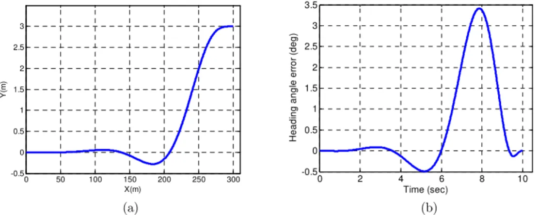
Similar to the first simulation, the path planning program uses the above lateral acceleration con-straint for solving the boundary value problem. Lateral deviation of the optimal path from the ref-erence path versus the distance vehicle travels along the refref-erence path is shown in Figure 8(a) and heading angle error of the optimal path from the reference path is shown in Figure 8(b). It can be seen that on the circular road, the autonomous vehicle carries out the lane-change maneuver earlier than when it moves on the straight road due to the lower value of lateral acceleration constraint with respect to the first case. The output of the program is the control input and states x and y

for generating the path. Since y demonstrates deviation of the optimal path from the reference

path, the variable y should be added to the reference path to generate the target path for the

vehi-cle to follow.

(a) (b)

Figure 8: Path planning results: a) lateral deviation of the optimal path from the reference path versus the distance

along the reference path, b) lateral acceleration (g) of vehicle for performing the lane-change maneuver on circular road.

0 50 100 150 200 250 300

-0.5 0 0.5 1 1.5 2 2.5 3

X(m)

Y(

m

)

0 2 4 6 8 10

-0.5 0 0.5 1 1.5 2 2.5 3 3.5

Time (sec)

H

eadi

ng angl

e er

ror

(

(16)

By importing the lateral deviation of the optimal path with respect to the reference path into the CarSim, the software solver combines the input with the reference path and generates the target path for the CarSim vehicle model to follow it. Figure 9(a) shows the target optimal path, reference circular path and path tracked by the vehicle during executing the overtaking maneuver. For a clearer view, only the section of overtaking maneuver of the path is shown. Similar to the case of moving on the straight road, the vehicle tracks the regenerated optimal path with small tracking errors. Figure 9(b) shows the actual steering angle of front wheels for performing the double lane-change maneuver. It can be seen that the vehicle has about 0.4 deg steering angle for moving on the reference path and maximum 1.2 deg for accomplishing the double lane-change maneuver. Figure 9(c) shows the actual lateral acceleration of the autonomous vehicle during the overtaking maneu-ver. As demonstrated in Figure 9(c), the vehicle has the lateral acceleration of 0.18g before starting the double lane-change maneuver and after accomplishing the maneuver, the lateral acceleration of vehicle doesn’t exceed 0.3g which means that the autonomous vehicle can track the target path generated by the bicycle model with similar dynamic behavior.

(a)

(b) (c)

Figure 9: Path tracking results: a) target, reference and actual path of vehicle b) actual lateral acceleration of

vehi-cle (g) during the overtaking maneuver on the circular road.

150 200 250 300 350

50 100 150 200

Global x coordinate (m)

G

loba

l y

c

oo

rd

ina

te

(m

) Target path

Reference path Vehicle path

0 2 4 6 8 10 12 14 16 18 20

-0.5 0 0.5 1 1.5 2

Time (sec)

St

e

ri

ng

an

gl

e (

d

e

g

)

0 2 4 6 8 10 12 14 16 18 20

0 0.05 0.1 0.15 0.2 0.25 0.3 0.35

Time (sec)

La

te

ra

l acce

le

ra

tion

(

g

(17)

4 CONCLUSIONS

This study presents a global optimal path planning of an autonomous vehicle for overtaking a mov-ing obstacle. The path plannmov-ing program is presented for generatmov-ing the optimal path of vehicle for performing the lane-change maneuver when it approaches a slow moving vehicle which is considered as an obstacle. It generates the path in such way that the sum of the lateral deviation of vehicle from the reference path and the rate of steering angle become minimum. The vehicle dynamics con-straint and the lateral acceleration inequality concon-straint were used to prepare the nonlinear optimal control problem of path planning program to generate the path by using Pontryagin’s Minimum Principle and the optimal path is generated as the global optimal solution. In addition, the CarSim software is used for the path tracking simulation by importing the path data from MATLAB re-sults. The simulation results show that the autonomous vehicle can track the generated path and satisfies all vehicle dynamic constraints and hence is suitable to overtake the leading vehicle. The solution, however, shows that the path has an unexpected deviation from the reference path to the opposite direction when the optimal control problem with only one cost function is used. The solu-tion with two cost funcsolu-tions will be examined in the future.

References

Arras, K. O., Persson, J., Tomatis, N., Siegwart, R., (2002). Real-time obstacle avoidance for polygonal robots with a reduced dynamic window. IEEE International Conference on Robotics and Automation, Washington D.C.

Borrelli, F., Falcone, P., Keviczky, T., Asgari, J., Hrovat, D., (2005). Mpc-based approach to active steering for autonomous vehicle systems. International Journal of Vehicle Autonomous Systems 3(2/3/4): 265–291.

Garg, D., Hager, W., Rao, A. V., (2011). Pseudospectral methods for solving infinite-horizon optimal control prob-lems. Automatica 47(4): 829-837.

Isermann, R., Schorn, M., Stählin ,U., (2008). Anticollision system proreta with automatic braking and steering. International Journal of Vehicle Mechanics and Mobility 46(S1): 683-694.

Kim, W., Kim, D., Yi, K., Kim, H.J., (2011). Development of a path-tracking control system based on model predic-tive control using infrastructure sensors. Vehicle System Dynamics 50(6): 1001-1023.

Kirk, D. E., (2004). Optimal control theory: An introduction. Donver Publication, Inc. (Mineola , New York). Mashadi, B., Ahmadizadeh, P., Majidi, M., Mahmoodi-Kaleybar, M., (2014). Integrated robust controller for vehicle path following. Multibody System Dynamics: 1-22.

Matveev, A. S., Teimoori, H., Savkin , A. V., (2011). A method for guidance and control of an autonomous vehicle in problems of border patrolling and obstacle avoidance. Automatica 47(3): 515-524.

Minguez, J., Montano, L., (2005). Sensor-based robot motion generation in unknown, dynamic and troublesome scenarios. Robotics and Autonomous Systems 52(4): 290-311.

Nanao, M., Ohtsuka, T., (2010). Nonlinear model predictive control for vehicle collision avoidance using c/gmres algorithm. IEEE International Conference on Control Applications, Yokohama, Japan.

Naranjo, J. E., González, C., García, R., Pedro, T.D., (2008). Lane-change fuzzy control in autonomous vehicles for the overtaking maneuver. IEEE Transactions on Intelligent Transportation Systems 9(3): 438-450.

(18)

Park, J.M., Kim, D.W., Yoon, Y.S., Kim, H. J., Yi, K.S., (2009). Obstacle avoidance of autonomous vehicles based on model predictive control. Proc IMechE, Part D: J Automobile Engineering 223: 1499-1516.

Park, J., Kim, D., Yoon, Y., Kim, H., Yi, K., (2009). Obstacle avoidance of autonomous vehicles based on model predictive control. Proc. IMechE, Part D: Journal of Automobile Engineering 223(12): 1499-1516.

Purwin, O., D’Andrea, R., (2006). Trajectory generation and control for four wheeled omnidirectional vehicles. Ro-botics and Autonomous Systems 54(1): 13-22.

Rashid, A. T., Ali, A. A., Frasca, M., Fortuna, L., (2013). Path planning with obstacle avoidance based on visibility binary tree algorithm. Robotics and Autonomous Systems 61(12): 1440-1449.

Spenko, M., Iagnemma, K. D., Dubowsky, S., (2004). High speed hazard avoidance for mobile robots in rough ter-rain. SPIE conference on unmanned ground vehicle technology, Orlando, FL.

Wang, X., (2009). Solving optimal control problems with matlab: Indirect methods.

Yahja, A., Singh, S., Stentz, A., (2000). An efficient on-line path planner for outdoor mobile robots. Robotics and Autonomous Systems 32(2–3): 129-143.

Yoon, Y., Shin, J., Kim, H. J., Park, Y., Sastry, S., (2009). Model-predictive active steering and obstacle avoidance for autonomous ground vehicles. Control Engineering Practice 17(7): 741-750.

Yuan, H., Yang, J., Qu, Z., Kaloust, J., (2006). An optimal real-time motion planner for vehicles with a minimum turning radius. the 6th World Congress on Intelligent Control and Automation, Dalian, China.