ABSTRACT: This paper presents the simulation results of an aeroassisted maneuver around the Earth, between coplanar circular orbits, from a geostationary orbit to a low orbit. The simulator developed considers a reference trajectory and a trajectory perturbed by external disturbances combined with non-idealities of sensors and actuators. It is able to operate in closed loop, controlling the trajectory (drag-free control) at each instant of time using a Proportional-Integral-Derivative (PID) controller and propulsive jets. We adopted a spacecraft with a cubic body composed of two rectangular plates arranged perpendicular to the velocity vector of the vehicle. Propulsive jets are applied at the apogee of the transfer orbit in order to keep the perigee altitude and control the rate of heat transfer suffered by the vehicle during atmospheric passage. A PID controller is used to correct the deviation in the state vector and in the keplerian elements. The U.S. Standard Atmosphere is adopted as the atmospheric model. The results have shown that the aeroassisted transfer presents a smaller fuel consumption when compared to a Hohmann transfer or a bi-elliptic transfer.
KEYWORDS: Aeroassisted maneuvers, Orbital dynamic, Trajectory control.
Trajectory Control During an Aeroassisted
Maneuver Between Coplanar Circular Orbits
Willer Gomes dos Santos1, Evandro Marconi Rocco1, Valdemir Carrara1INTRODUCTION
An orbital maneuver is the transfer of a satellite from one orbit to another by means of a change in velocity. To perform this change, the spacecrat has to engage the thrusters or use the natural forces of the environment. he Hohmann transfer and the bi-elliptic transfer are some alternatives to perform an orbital maneuver by propulsive means. In 1961, Howard London presented the approach of using aerodynamic forces to change the trajectory and velocity of a spacecrat, this new technique became known as aeroassisted maneuvers (Walberg, 1985). his type of orbital transfer can be accomplished in several layers of the atmosphere. he altitude reached by vehicle is linked to the mission’s purpose and to the maximum thermal load supported by the vehicle structure. he main advantage of this type of maneuver is the fuel economy. According to Walberg (1985), many papers on aeroassisted orbital transfer have been made in recent decades and it has been shown that a signiicant reduction in fuel can be achieved using aeroassisted maneuvers instead of Hohmann transfer. Consequently, the reduction of fuel provides an increase in the payload capacity of the vehicle. Orbit transfer between two circular and coplanar orbits is very common. he technique of using atmospheric drag to reduce the semi-major axis is known as aerobraking and it was irst used on March 19th, 1991, by spacecrat Hiten. he launch was conducted
by the Institute of Space and Astronautical Science of Japan (ISAS). he spacecrat passed through Earth’s atmosphere at an altitude of 125.5 km over the Paciic Ocean at a speed of 11 km/s. he experience resulted in a decrease in apogee altitude of 8,665 km. In May 1993, an aerobraking maneuver was used on a mission to Venus by Magellan spacecrat, whose goal was to circularize the orbit of the spacecrat. In 1997, the probe U.S. Mars Global Surveyor (MGS)
1.Instituto Nacional de Pesquisas Espaciais – São José dos Campos/SP – Brazil
Author for correspondence: Willer Gomes dos Santos | Instituto Nacional de Pesquisas Espaciais | Avenida dos Astronautas 1758, São José dos Campos/SP | CEP: 12227-010 – Brazil | Email: [email protected]
used its solar panels as “wings” to control its passage through the tenuous upper atmosphere of Mars and lower its apoapsis.
here are several missions requirements that become feasible with the use of aeroassisted vehicles, as for example, to reconigure orbital systems that are unable to perform an orbital maneuvering (such as replacing a malfunctioning satellite by a spare), to transfer space debris to a new orbit, to operate Space Transportation Systems (STS), to use the atmospheric drag as a brake force to provide orbit capturing of the vehicle, to assist the International Space Station with the transfer of cargo between geostationary orbit (GEO) and low earth orbit (LEO), among others.
Within the context of this paper, we can cite the scientiic micro-satellite Franco-Brazilian (FBM) project, in partnership between the Brazilian and French space agencies (INPE and CNES), which would be released as piggy-back on an Ariane 5, and then would perform aerobraking maneuvers to transfer the satellite to the orbit service (Furlan, 1998). he Ariane 5 rocket has the capacity to carry up to eight microsatellites with a maximum individual weight of 120 kg through the Ariane Structure for Auxiliary Payload (ASAP). However, the rocket was designed to place satellites in geostationary transfer orbits. he propellant required to transfer the FBM to a low orbit (between 800 and 1,300 km) by means of chemical propellants, would exceed the allowed amount of mass. his question has led space agencies to study the concept of aerobraking as a workaround. However, CNES, in 2003, let the program which was subsequently discontinued (Brezun et al., 2000). In another interesting study with the same context, Schulz (2001) developed an optimal control law that minimizes the fuel consumption during an aeroassisted maneuver, as well as analyzed orbital changes.
his paper will present the simulation of an aerobraking maneuver between GEO and low orbit. The study aims at examinining the efects that this kind of maneuver can cause in the orbital elements. It will also demonstrate the diference in fuel costs and the elapsed transfer time between an aeroassisted maneuver and a fully propulsive maneuver. he results show that the aeroassisted transfer has a propellant consumption lower than a Hohmann or a bi-elliptic transfer.
PROBLEM DEFINITION
In this paper, a spacecrat with a cubic body composed of two rectangular plates was adopted, called aerodynamic plates,
placed in opposite sides of the vehicle’s body. he inclination angle of the plates, regarding its molecular low (attack angle), was ixed at 90 degrees, in order to maximize the projected area and the drag force. he spacecrat will be transferred from the GEO to a low orbit. he orbits are considered circular and coplanar. A multipass aeroabraking strategy is used to perform the transfer.
First, the spacecrat applies an impulse to take the vehicle out of the GEO and put it into an elliptical orbit with perigee within the limits of the atmosphere. Ater each passage at atmospheric region, a reduction of the apogee transfer orbit occurs. When the spacecrat reaches its inal apogee altitude, then, a new impulse is applied to the vehicle to remove it from the transfer orbit and insert it into the inal orbit. In order to control the rate of heat transfer sufered by the vehicle during the passage through atmosphere, propulsive jets are applied at the apogee, correcting the decay of perigee. his transfer strategy is shown in Fig. 1.
Figure 1. Multipass aerobraking (Walberg, 1985).
deorbit (OTV)
Atmosphere Limit
Target Orbit (LEO FOR OTV) Final circularization and periapsis raise maneuver
Apoapsis trim maneuvers to adjust periapsis
GEO
of sensors and actuators. he simulator works in closed loop controlling the trajectory at each instant of time, which is one of the input parameters, using a Proportional-Integral-Derivative (PID) controller and propulsive jets. Santos (2011) used the SAMS to study how the orbital elements can be changed by an aeroassisted maneuver and how much fuel is saved comparing with a propulsive maneuver. Figure 2 shows a basic diagram of the running logic of the aeroassisted maneuver simulator. In this work, noises and non-idealities in the actuator and in the sensor were not considered.
According to heil and Silas-Guilherme (2005), drag-free technology is essential for scientiic missions which need a very low disturbance environment. Several missions have used this technology, such as Gravity Probe B (GP-B) to test the relativistic efects on a gyroscope; STEP and MICROSCOPE had the objective of testing the weak principle of equivalence; Laser Interferometer Space Antenna (LISA) for the detection of gravitational waves; and Gravity Field and Steady State Ocean Circulation Explorer (GOCE), launched in March 2009, to determine the gravity-ield anomalies with high accuracy; among others.
AEROASSISTED MANEUVER
he main forces acting on a spacecrat in LEO are gravitational force (mg), thrusters force (Ts) and aerodynamic forces (F), caused by the interaction of the satellite with the atmosphere. he spacecrat position in space determines the magnitude of aerodynamic forces sufered by the spacecrat. he higher the planetary atmospheric density is, the stronger the aerodynamic forces are. he aerodynamic force can be divided into two: the drag force (FD), whose direction is opposite to the velocity vector, and the lit force (FL), perpendicular to the drag force. According to Vinh (1981), the magnitude of these forces is given by the following equations:
(1)
(2)
where r is the atmosphere density, CD and CL are, respectively, the drag and lit coeicients on the projected area S, and V is the velocity of the spacecrat in relation to the atmosphere. he lit can also be decomposed into altitude lit force (FA) and lateral lit force (FB). he attack angle (a ) is measured between the longitudinal axis of the spacecrat and velocity in relation to the atmosphere. he magnitude of the aerodynamic force depends mainly on the attack angle, and its direction varies depending on the bank angle (s ) between the lit plane and the plane, formed by the velocity vector in relation to the atmosphere and the vector position of the spacecrat, as shown in Fig. 3.
he direction and amplitude of these forces can be calculated by the following equations (Guedes, 1997):
(3)
Figure 2. Basic diagram of the aeroassisted maneuver simulator.
Disturbance
Disturbed state Orbital Dynamic Reference
State
PID Controller
Sensor Propulsive
System +
-+ +
BACKGROUND CONCEPTS
his section aims at presenting the main equations and concepts used in the development of this work. Firstly, the concepts about drag-free technology are presented, and then the equations of aeroassisted maneuver and trajectory control system are introduced.
THE DRAG-FREE SATELLITE
(4)
where is the velocity in relation to the atmosphere versor; is the angular momentum versor; and is the altitude versor. he altitude lit force, the lateral lit force, the angular momentum vector and the altitude vector are calculated according to the following equations:
(5)
(6)
H = R×V (7)
N = V×H (8)
The drag coefficient (CD), altitude lift (CA) and lateral lift (CB), are calculated using the Impact Method (Regan and Anandakrishnan, 1993), according to the following equations:
CD = 2sen2α (9)
CL = 2senα cosα (10)
CA = CLcosσ (11)
CB = CLsenσ (12)
he Impact Method, or Newtonian Impact heory (Vinh et al., 1970), is a simpliied numerical technique to approximate the forces and torques acting on a body. It assumes an elastic relection of particles in a specular surface. he normal component of impact velocity is reversed while the tangential component is unchanged. his model assumes that the particles have no random velocity component, usually associated to microscopic particles of gas (Regan and Anandakrishnan, 1993).
he U.S. Standard Atmosphere model provides the value of the atmospheric density, depending on the position of the vehicle, for the calculation of aerodynamic forces. he velocity of the spacecrat in relation to the atmosphere in the inertial system is calculated assuming that the atmosphere has the same rotation velocity of the Earth and its equation is given by Kuga et al. (2008):
(13)
where is the velocity vector in relation to the inertial system and ω is the angular velocity vector of Earth’s rotation.
Some of the major diiculties faced by the spacecrat during atmospheric maneuver are related to the heating rate and velocity deceleration. hese quantities increase when the vehicle is submitted to high atmospheric densities and high velocities. In the upper atmosphere, it should be considered a form of heating known as free molecular heating. his phenomenon occurs due to the impact of free molecules against the vehicle. he rate of heat transfer as per area unit is given by the following equation (Gilmore, 1994):
(14)
where αc is the thermal accommodation coeicient (Gilmore (1994) recommends the use of αc = 1).
he orbital spacecrat state is described by the coordinates
X = [r V], measured in an inertial frame centered on Earth, and the dynamic model of the spacecrat used in this paper is given by:
(15)
where μ is the central body gravitational constant (product of the central body mass and the universal gravitational constant)
Figure 3. Components of the aerodynamic forces, attack angle and bank angle (Guedes, 1997).
σ α
LONGITUDINAL AXIS
FL
FA
V
FB
FD
and ΔVp is the velocity variation caused by propulsive thrusters when activated. he lit force is null because the attack angle of the aerodynamic plates is perpendicular to the velocity vector.
TRAJECTORY CONTROL SYSTEM
A PID controller was used to correct the deviation of the spacecrat trajectory. Most of the industrial controllers are PID due to its lexibility, low cost and robustness. he PID control action is computed by:
(16)
where KP , KI and KD are the proportional gain, integral gain and derivative gain respectively, and e(t) is the position error. Most control systems today use digital computers. Hence, to implement the PID control law in a digital computer, it is necessary to discretize the PID equation c(t). Several discretization methods can be consulted in Franklin et al. (1998). Using the discretization methodology proposed by Hemerly (2000), we can write the discrete PID control law equation, as
(17)
where T is the sample period.
RESULTS
his section aims at presenting the results of an aeroassisted maneuver simulation to transfer the spacecrat from a GEO to a low orbit of 1,000 km of altitude. he presented curves refer only to the aeroassisted transfer. Table 1 shows the initial conditions of the orbit. he complete maneuver was performed in 58.93 days and, at the end of the period, there was a reduction of approximately 35,000 km in the apogee altitude, according to Fig. 4. The perigee altitude remained at an average of 115 km, with a variation of ± 0.5 km due to the application of jet propulsion at the apogee of the orbit, shown in Fig. 5.
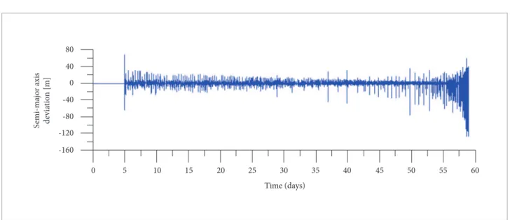
here was no change in the orbit inclination because lit forces were not being applied to the vehicle. Figure 6 illustrates
Table 1. Initial condition of the transfer orbit.
Description Value Units
Apogee altitude 35786.14 km
Perigee altitude 115 km
Eccentricity 0.7332
-Inclination 1 degrees
RAAN* 200 degrees
Perigee argument 10 degrees
Mean anomaly 180 degrees
*Right Ascension of Ascending Node.
Figure 4. Apogee altitude as function of time. 0
0
A
p
og
ee a
lt
it
ude [k
m]
40000
20000 30000
10000
10
5 15 20
Time (days)
Figure 5. Perigee altitude as function of time. 100
0
P
er
ig
ee a
lt
it
ude [k
m]
120
110 115
105
10
5 15 20
Time (days)
25 30 35 40 45 50 55 60
Figure 6. Semi-major axis deviation as function of time. -120
0
S
emi-m
aj
o
r axi
s
de
vi
at
io
n [m]
80
-40 40
-80
10
5 15 20
Time (days)
25 30 35 40 45 50 55 60
-160 0
the deviation of the semi-major axis versus time. During the maneuver, the control system acts to reduce the error between the reference trajectory and the disturbed trajectory. he error appears when the irst thrust is applied at the apogee.
Figure 7 shows the variation in the position components X, Y and Z, for the irst ive days of maneuvering. he variation is almost zero at the Z component due to the roughly equatorial orbit. he behavior X and Y components is related to the orbit eccentricity. As the vehicle approaches the perigee the orbital velocity increases, and vice versa.
he applied thrust at the orbit apogee versus time is shown in Fig. 8. Due to orbit circularization the trajectory path inside
low atmosphere is increased, causing perigee decay. So, while low thrusters are applied at the beginning of the maneuvering process in order to adjust the trajectory derivations, high impulses are employed at the inal orbit to correct the perigee height.
Figure 9 illustrates the drag force sufered by the vehicle along the atmospheric path. It can be observed a downward trend close to the inal orbit. his behavior is related to the velocity reduction and with the circularization of the orbit.
Figure 7. X, Y and Z components of the position and velocity vectors as function of time.
0
Y p
osi
tio
n [m] 4E+007
-2E+007 2E+007
-4E+007
1
0.5 1.5 2
Time (days)
2.5 3 3.5 4 4.5 5
6E+007 0E+000 0 Z p osi tio
n [m] 4E+007
-2E+007 2E+007
-4E+007
10
5 15 20
Time (days)
25 30 35 40 45 50
6E+007 0E+000 55 60 0 X v elo ci ty [m/s] 10000 -5000 5000 -10000 1
0.5 1.5 2
Time (days)
2.5 3 3.5 4 4.5 5
15000 0 -15000 0 Y v elo ci ty [m/s] 10000 -5000 5000 -10000 1
0.5 1.5 2
Time (days)
2.5 3 3.5 4 4.5 5
15000
0
-15000
0 5 10 15 20
Time (days)
25 30 35 40 45 50 55 60
Z v elo ci ty [m/s] 10000 -5000 5000 -10000 15000 0 -15000 0 X p osi tio
n [m] 4E+007
-2E+007 2E+007
-4E+007
1
0.5 1.5 2
Time (days)
2.5 3 3.5 4 4.5 5
6E+007 0E+000 0 0 Thr u st [N] 1.6 0.8 1.2 0.4 10
5 15 20
Time (days)
25 30 35 40 45 50 55 60
Figure 8. Propulsive thrust as function of time.
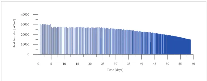
the heat rate experienced by the vehicle can be increased or decreased by controlling the perigee altitude; the lower the perigee height, the higher the heat sufered by the vehicle.
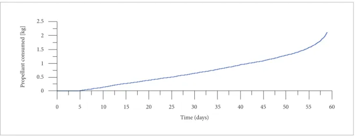
Regarding the consumption of propellant, two situations are considered. he irst one illustrates a hypothetical situation: it is considered that the drag force sufered by the vehicle is
provided by the propulsion system, whose results are presented in Fig. 11; and the second situation (Fig. 12), shows the case that considers only the thrust necessary to correct the perigee altitude.
0
0
H
ea
t t
ra
n
sf
er [W/m
2]
40000
20000 30000
10000
10
5 15 20
Time (days)
25 30 35 40 45 50 55 60
Figure 10. Rate of heat transfer as function of time.
0
0
P
ro
p
el
la
n
t co
n
sum
ed [kg]
250
150 200
50
10
5 15 20
Time (days)
25 30 35 40 45 50 55 60
100
Figure 11. Hypothetical situation: propellant required for applying a thrust equal to drag force.
0
Dra
g f
o
rce [N]
0
-20 -10
-30
10
5 15 20
Time (days)
25 30 35 40 45 50 55 60
Table 2. Comparative table of propellant consumption and transfer time.
Maneuvers Propellant Consumption (kg)
Transfer time (days)
Hohmann 276.62 0.22
Bi-elliptic 361.25 1.48
Aeroassisted 160.92 58.93
0
0
P
ro
p
el
la
n
t co
n
sum
ed [kg]
2.5
1.5 2
0.5
10
5 15 20
Time (days)
25 30 35 40 45 50 55 60
1
Figure 12. Aeroassisted situation: propellant necessary to correct the decay of perigee.
transfer, compared to 2.11 kg of fuel, necessary to the aeroassisted, plus PID control orbit maneuvering. Furthermore, it should be taken into account the propellant needed to enter to and exit from the transfer elliptical orbit. he propellant adopted was the liquid oxygen/liquid hydrogen, whose speciic impulse is 460 s. Table 2 shows a comparison of propellant consumption and transfer time among Hohmann transfer, Bi-elliptic transfer and aeroassisted maneuver. It was considered the consumption of propellant to enter and to exit from the elliptical orbit transfer. he aeroassisted maneuver spent 160.92 kg of propellant, where 2.11 kg were used to correct the decay of perigee, and 158.81 kg to get in and out of the transfer orbit. he fuel economy of aeroassisted maneuver related on the transfer of Hohmann was approximately 116 kg.
in computations, the ideal case for calculating the transfer time of propulsive maneuvers, but when thrust is small, due to thruster size, and the number of propulsive maneuvers to reach the inal orbit is increased, the time to perform the maneuver also increases.
CONCLUSIONS
It was presented the simulation of an aeroassisted maneuver to transfer a vehicle from a GEO to a low orbit altitude using propulsive jets to correct the decay in perigee altitude and to correct deviations between the reference trajectory and the disturbed trajectory. It can be concluded that the control system met expectations and that it has maintained the residual error in state vector within acceptable limits.
he control propulsive jets is able to maintain the perigee altitude within reasonable limits (115 km ± 0.5 km), avoiding the vehicle to sufer high thermal loads during the atmospheric path. his case can be compared to the mission of scientiic FBM, in which there was a need to transfer the satellite from a GEO to a low orbit, by means of aeroassisted maneuvers. In general, the aeroassisted maneuvers were more advantageous in terms of fuel economy than the fully propulsive maneuvers. he closed loop control system was critical to the simulation success, without which it would not be possible to eliminate eiciently the residual errors in the trajectory.
REFERENCES
Brezun, E., Bondivenne, G. and Kell, P., 2000, “Aerobraking design and study applied to CNES microsatellite product line”, 5th International Symposium of Small Satellites Systems and Services, La Baule, France. Proceedings… Paris: CNES, 2000. pp. 673-680.
Franklin, G.F., Powell, J.D. and Workman, M.L., 1998, “Digital Control of dynamic systems”, 3rd Edition, Addison-Wesley Publishing Co., Massachusetts, USA
Furlan, B.M.P., 1998, “Several studies apply to the French-Brazilian mission”, Instituto Nacional de Pesquisas Espaciais (INPE), São José dos Campos, Brazil (in Portuguese).
Gilmore, D.G., 1994, “Satellite thermal control handbook”, 1st Edition, The Aerospace Corporation Press, California, USA.
Guedes, U.T.V., 1997, “Dispersion analysis of the reentry trajectory over the landing point, using geocentric inertial and lateral maneuvers”, Ph.D. in Space Mechanics and Control Thesis, Instituto Nacional de Pesquisas Espaciais (INPE), São José dos Campos, Brazil (in Portuguese).
Hemerly, E.M., 2000, “Controle por computador de sistemas dinâmicos”, 2nd Edition, Edgard Blücher Ltda, São Paulo, Brazil.
Kuga, H.K., Rao, K.R. and Carrara, V., 2008, “Introduction to Orbital Mechanics” 2nd Edition, Instituto Nacional de Pesquisas Espaciais (INPE), São José dos Campos, Brazil (in Portuguese).
Kumar, M. and Tewari, A., 2005, “Trajectory and attitude simulation for aerocapture and aerobraking”, Jornal of Spacecraft and Rockets, Vol. 42, No. 4, pp. 684-693. doi: 10.2514/1.7117.
Regan, F.J. and Anandakrishnan, S.T., 1993, “Dynamics of atmosphere re-entry”, 1st Edition, American Institute of Aeronautics and Astronautics, Washington, DC, USA.
Rocco, E.M., 2006, “Tools for analysis and simulation of spacecraft trajectories in keplerian orbit” Bremen: Center of Applied Space Technology and Microgravity ZARM, University of Bremen, Germany.
Rocco, E.M., 2008, “Perturbed orbital motion with a PID control system for the trajectory”, XIV Colóquio Brasileiro de Dinâmica Orbital, Águas de Lindóia, Brazil.
Rocco, E.M., 2009, “Earth albedo model evaluation and analysis of the trajectory deviation for some drag-free missions”, Proceedings of the 8th Brazilian Conference on Dynamics Control and Applications, Bauru, Brazil.
Rocco, E.M., 2010, “Evaluation of the terrestrial albedo applied to some scientiic missions”, Space Science Reviews, Vol. 151, No. 1-3, pp. 135-147. doi: 10.1007/s11214-009-9622-6, 2010.
Santos, W.G., 2011, “Simulação de manobras aeroassistidas de um veículo espacial controlado por placas aerodinâmicas reguláveis e sistema propulsivo”, Dissertação de Mestrado em Mecânica Espacial e Controle, Instituto Nacional de Pesquisas Espaciais (INPE), São José dos Campos, Brazil, pp. 272.
Schulz, W., 2001, “Study of orbital transfers including aeroassisted maneuvers” Ph.D. in Space Mechanics and Control Thesis, Instituto Nacional de Pesquisas Espaciais (INPE), São José dos Campos, Brazil, pp. 178 (in Portuguese).
Theil, S. and Silas-Guilherme, M., 2005, “In-orbit calibration of drag-free satellites”, Advances in Space Reseach, Vol. 36, pp. 504-514. doi: 10.1016/j.asr.2005.05.126.
Vinh, N.X., Busemann, A. and Culp, R.D., 1970, “Hypersonic and planetary entry light mechanics” Elsevier, Amsterdam, Germany.
Vinh, N.X., 1981, “Optimal trajectories in atmospheric light” Elsevier, Amsterdam, Germany.


![Figure 7. X, Y and Z components of the position and velocity vectors as function of time.0Y position [m]4E+007-2E+0072E+007-4E+00710.51.52Time (days)2.533.544.556E+0070E+0000Z position [m]4E+007-2E+0072E+007-4E+0071051520Time (days)2530354045506E+0070E+000](https://thumb-eu.123doks.com/thumbv2/123dok_br/18889351.424632/7.892.84.809.134.542/figure-components-position-velocity-vectors-function-position-position.webp)