Sports analytics: maximizing precision in predicting MLB base hits

(1)

SPORTS ANALYTICS: MAXIMIZING PRECISION IN

PREDICTING MLB BASE HITS

Pedro Miguel Gonçalves André Alceo

Dissertation presented as the partial requirement for

obtaining a Master's degree in Information Management

(2)

NOVA Information Management School

Instituto Superior de Estatística e Gestão de Informação

Universidade Nova de Lisboa

SPORTS ANALYTICS: MAXIMIZING PRECISION IN PREDICTING MLB

BASE HITS

Pedro Miguel Gonçalves André Alceo

Dissertation presented as the partial requirement for obtaining a Master's degree in Information Management, Specialization Knowledge Management and Business Intelligence Advisor: Roberto André Pereira Henriques

February 2019

(3)

iii

ACKNOWLEDGEMENTS

The completion of this master thesis was the culmination of my work accompanied by the endless support of the people that helped me during this journey. This paper would feel emptier without somewhat expressing my gratitude towards those who were always by my side.

Firstly, I would like to thank my supervisor Roberto Henriques for helping me find my passion for data mining and for giving me the guidelines necessary to finish this paper. I would not have chosen this area if not for you teaching data mining during my master’s program.

To my parents João and Licínia for always supporting my ideas, being patient and for along my life giving the means to be where I am right now. My sister Rita, her husband João and my nephew Afonso, whose presence was always felt and helped providing good energies throughout this campaign.

To my training partner Rodrigo who was always a great company, sometimes an inspiration but in the end always a great friend. My colleagues Bento, Marta and Rita who made my master’s journey unique and very enjoyable. To my closest friends who have accompanied me throughout my life that are too many to name but have always provided a great environment for companionship and self-growth.

(4)

iv

RESUMO

Nos últimos anos o mundo do desporto alcançou níveis de crescimento nunca antes visto e, este evento, fomentou a necessidade para o crescimento no uso de ferramentas que tragam vantagens para as organizações e os respetivos stakeholders. Como resultado tem se registado um rápido crescimento no uso da análise de dados para vários tópicos relacionados com o desporto que consequentemente origina melhores e rápido julgamentos para os tomadores de decisão.

Nesta linha de pensamento, o principal objetivo deste projeto é contruir um modelo preditivo capaz de prever as probabilidades de um jogador da MLB obter um “base hit” num dia com o propósito de ganhar o jogo Beat the Streak e, ao mesmo tempo, providenciar informações valiosas à equipa técnica.

A arquitetura que serviu de diretriz a este projeto foi o CRIPS-DM, o qual foi aplicado a uma base de dados construída especificamente para este projeto com dados publicamente acessíveis. Para alcançar os referidos objetivos, foram usados o Excel com meio para recolher e estruturar a base de dados e o Python para os restantes processos com um enfase na biblioteca SKlearn. Os elementos que separam as construções dos modelos finais foram o balanceamento da base de dados, outliers, redução da dimensionalidade, seleção das variáveis e os algoritmos – Logistic Regression, Multi-layer

Perceptron, Random Forest e Stochastic Gradient Descent.

Os resultados obtidos foram positivos sendo o modelo com a melhor performance um Multi-layer Perceptron que obteve 85% de escolhas certas no set de teste. Este resultado alcançou uma melhoria de 5 pontos percentuais sobre o melhor modelo encontrado durante a pesquisa bibliográfica.

Os resultados em questão foram positivos, mas existe margem para melhorar os modelos desenvolvidos ou a criação de outros modelos porque com os resultados obtidos ainda é difícil ganhar o jogo Beat the Streak, o que deixa em aberto a possibilidade para a criação de novos modelos.

PALAVRAS-CHAVE

(5)

v

ABSTRACT

As the world of sports expanded to never seen levels, so did the necessity for tools which provided material advantages for organizations and other stakeholders. This resulted in an increase on the use of data and analytics for a multitude of sports related topics, which led to more precise and quicker judgements for decision makers related to sports.

In this line of though, the main objective of this paper is to build a predictive model capable of predicting what are the odds of a baseball player getting a base hit on a given day, with the intention of both winning the game Beat the Streak and to provide valuable information for the coaching staff. CRISP-DM was the architecture chosen as the main guideline to apply on the dataset, entirely built for this paper, using publicly available data. To achieve these objectives, Excel was used for data collection purposes and Python for the remaining steps with a big emphasis on the SKlearn library. Several models were tested and the main constrains that separate them from each other are balancing, outliers, dimensionality reduction, variable selection and the type of algorithm – Logistic Regression, Multi-layer Perceptron, Random Forest and Stochastic Gradient Descent.

The results obtained were positive, in which one of the Multi-layer Perceptron achieved an 85% correct pick ratio on the test set, which is an improvement of 5 percentage points over the best model found during the literature review.

Nevertheless, there is undoubtedly room for improvements in the final models and for other models with similar intentions, since the results achieved do not provide a good change of Beating the Streak.

KEYWORDS

(6)

vi

INDEX

1. Introduction ... 1

1.1. Context and Relevance ... 1

1.2. Problem ... 1

1.3. Objective ... 2

1.4. Study Outline ... 3

2. Literature Review ... 4

2.1. Data Mining ... 4

2.2. Sports Analytics ... 5

2.2.1. Evolution of Sports Analytics ... 5

2.2.2. Data Mining in Sports ... 6

2.3. Baseball Analytics ... 7

2.3.1. State of Data Mining in Baseball ... 8

2.3.2. Statcast ... 9

2.3.3. Predicting batting performance ... 10

3. Methodology ... 13

3.1. Data Collection ... 14

3.2. Data Understanding ... 15

3.2.1. Category description ... 15

3.2.2. Data Exploration ... 18

3.3. Data Preparation ... 25

3.3.1. Data sampling ... 25

3.3.2. Data partitioning ... 26

3.3.3. Data transformation ... 27

3.3.4. Missing values ... 29

3.3.5. Outliers ... 30

3.4. Modelling ... 31

3.4.1. Algorithms ... 31

3.4.2. Feature selection ... 33

3.4.3. Hyperparameter tuning ... 35

3.5. Evaluation ... 36

4. Results and Discussion ... 39

5. Conclusions ... 44

(7)

vii

7. References ... 47

8. Annexes ... 53

8.1. Modelling Evaluation Metrics for Validation Set ... 53

8.2. Modelling Evaluation Metrics for Test Set ... 54

8.3. Full Pearson’s Correlation Table ... 55

(8)

viii

LIST OF FIGURES

Figure 1 – CRISP-DM architecture ... 5

Figure 2: Luck in sports ... 7

Figure 3: Percentage of Sports organizations that use analytics, in North American Major

Leagues ... 8

Figure 4: Breakdown of a plate appearance ... 10

Figure 5: Literature review summary ... 12

Figure 6: Data sources and data management diagram ... 13

Figure 7: Top down model creation diagram ... 14

Figure 8: Pearson’s and Spearman’s correlation for target variable ... 21

Figure 9: Batting order influence on base hits ... 22

Figure 10: Number of games played by the batter influence on base hits... 22

Figure 11: Strikeouts influence on base hits ... 23

Figure 12: Opponent’s starting pitcher performance influence on base hits ... 23

Figure 13: ESPN Hit Factor influence on base hits ... 24

Figure 14: Ballparks displayed by ESPN Hit Factor and Altitude ... 24

Figure 15: Coors Field versus remaining ballparks, by base hit percentage ... 25

Figure 16: Average windspeed, ESPN Hit Factor and Altitude on ballparks, by type of roof .. 25

Figure 17: Data partitioning diagram ... 27

Figure 18: Boxplot example ... 31

Figure 19: RFE results by algorithm ... 34

Figure 20: Number of principal components features by summed explained variance ... 35

Figure 21: ROC Curve... 37

Figure 22: Average model performance on test set, by use of PCA ... 39

Figure 23: Variable usage, by type of feature selection ... 40

(9)

ix

LIST OF TABLES

Table 1: Beat the Streak scenario outcomes ... 10

Table 2: Sports Reference box-score display ... 15

Table 3: Variable description... 16

Table 4: Descriptive statistics for numeric variables ... 20

Table 5: Descriptive statistics for categorical variables ... 20

Table 6: Distribution of dependent variable ... 26

Table 7: Variable transformation description and calculations ... 28

Table 8: Example of variable encoding for the Roof Type Variable ... 29

Table 9: Hyper parameter tuning for the Logistic Regression ... 36

Table 10: Hyper parameter tuning for the Multi-layer Perceptron ... 36

Table 11: Hyper parameter tuning for the Random Forest ... 36

Table 12: Hyper parameter tuning for the Steep Gradient Descent ... 36

Table 13: Top 5 models evaluation metrics on validation set ... 41

Table 14: Top 5 models evaluation metrics on test set ... 41

Table 15: Threshold analysis on top 5 models ... 42

Table 16: Project results versus results of other strategies ... 43

LIST OF EQUATIONS

Equation 1: Probability of winning MLB beat the streak ... 2

Equation 2: Probability of winning MLB beat the streak ... 7

Equation 3: Batting Average and Hitting Percentage calculation ... 10

Equation 4: Min-Max Normalization Technique ... 28

Equation 5: Z-score formula ... 31

Equation 6: Cohen’s Kappa calculation ... 37

Equation 7: Precision calculation ... 37

(10)

x

LIST OF ABBREVIATIONS AND ACRONYMS

2B Double

AB At-Bat

AUC Area Under Curve BB Base-on-Balls

CRIPS-DM Cross Industry Standard Processes for Data Mining

H Hit

HBP Hit by Pitch HIP Hit in Play

HR Home Run

KDD Knowledge Discovery in Databases LG Logistic Regression

MLB Major League Baseball MLP Multi-Layer Perceptron

NBA National Basketball Association NFL National Football League NHL National Hockey League OBP On Base Percentage OIP Out in Play

PA Plate Appearance

PCA Principle Component Analysis

RC Runs Created

RF Random Forest

RFE Recursive Feature Elimination

SEMMA Sample, Explore, Modify, Model and Assess SGD Steep Gradient Descent

(11)

1

1. INTRODUCTION

“I’m sort of a baseball agnostic; I make it a point never to believe anything just because it is widely known to be so.” ― Bill James1

1.1. C

ONTEXT AND

R

ELEVANCE

In the past few years the professional sports market has been growing impressively. Events such as the Super Bowl, the Summer Olympics and the UEFA Champions League are fine examples of the dimension and global interest that can be generated by this industry currently. As the stakes grow bigger and further money and other benefits are involved in the market, new technologies and methods surge to improve stakeholder success (Mordor Intelligence, 2018).

The particular advancement most relevant for this project was the explosion of data creation and data storage systems, during the XXI century, which led to volumes of information that have never been so readily at our disposal before (Cavanillas, Curry, & Wahlster, 2016).Consequently, sports as many other industries could now use data to their advantage in their search for victory and, thus the sports analytics began its ascension to the mainstream (Gera et. All, 2016).

For most organizations winning is the key factor for good financial performance since it provides return in the form of fan attendance, merchandising, league revenue and new sponsorship opportunities (Collignon & Sultan, 2014). Sports analytics is a mean to reach this objective, by helping coaches, scouts, players and other personnel making better decisions based on data, leading to short and long-term benefits for stakeholders of the organization (Alamar, 2013).

The growing popularity of sports and the widespread of information also resulted in the growth of betting in sports events. This resulted in a growth of sports analytics for individuals outside sports organizations, as betting websites started using information based analytical models to refine their odds and gamblers to improve their earnings (Mann, 2018).

Finally, according to a study from Mordor Intelligence (2018) the sport who currently takes the most out of sports analytics is baseball. This is partially the consequence of historical events such as Moneyball where the use of analytics proved to have great effects in the outcome of the Oakland Athletics season, a baseball team which had the least money to spend on players in the League. For most, Moneyball was the turning point in analytics and baseball, which opened the way for the use of analytics in both baseball and other sports (Lewis, 2004).

1.2. P

ROBLEM

According to the MLB.com Glossary (MLB, 2018a), the definition of a base hit is:

“A hit occurs when a batter strikes the baseball into fair territory and reaches base without doing so via an error or a fielder's choice.”

1_{Bill James is an American baseball writer, historian and statistician (for more info go to}

(12)

2 A base hit is a common way for a player to reach a base and to advance other team mates already on base to potentially score runs. Therefore, base hits are among the best outcomes for batter, during his at-bat.

As easy as it sounds, batting the ball properly into the field of play is a big challenge even for professionals and, for examples, by taking the best batters from the 3 previous regular seasons (2015, 2016, 2017), in terms of hit% ([Hits/Plate Appearances]*100), we get Dee Gordon with 31,4%, Daniel Murphy with 31,6% and Jose Altuve with 30,8% respectively (Baseball Reference, 2018). In other words, for every attempt these batters had, they achieved a base hit only 31% of times. According to the dataset built for this paper around 66% of players (not accounting for pitchers batting) get at least one base hit during a game, which on average comprises 4 attempts per game (or plate appearances).

Additionally, during the 4 seasons comprised in the database or 9.720 games played the average streak was 2 and the 2 longest hitting streak achieved, allowing inter season streaks, was 28 by Jackie Bradley Jr. and 30 by Freddie Freeman. These reveals that picking the same player over and over may also not be a viable strategy.

For instance, to win the MLB Beat the Streak2_{it is required that the participant correctly picks 56}

times in row a player who gets a base hit in a given day. There are two important rules that should be considered. The first is that the maximum number of players one could pick in a single day is two, and the other is that it is not mandatory to make a pick every single day to keep the streak.

The main problem arises here, which in other words means that random guess does not provide a fair chance to win this game, which translated into a probability:

Equation 1: Probability of winning MLB beat the streak Source: Made by the author

1.3. O

BJECTIVE

The objective of this project is to build a database and a data mining model capable of predicting which MLB batters are most likely to get a base hit on a given day. In the end, the output of the work can have one of two uses:

1. To give a methodical approach for coach’s decision making and on what players should have an advantage on a given game and therefore make the starting lineup;

2. To improve one’s probabilities of winning the game MLB Beat the Streak.

For the construction of the database, it was collected data from the last four regular seasons of the MLB, from open sources. Regarding the granularity of the dataset, a sample consists on the variables of a player in a game. Additionally, in the dataset it was not considered pitchers batting nor players who had less than 3 plate appearances in the game. Finally, the main categories of the variables used in the models are:

(13)

3 • Batter Performance

• Batter’s Team Performance

• Opponent’s Starting Pitcher Performance • Opponent’s Bullpen Performance

• Weather • Ballpark

Regarding the batter’s performance those variables will include values from Statcast which is “a state-of-the-art tracking technology that allows for the collection and analysis of a massive amount of baseball data (…)” (MLB, 2018b). These stats in combination with a precision driven approach are what really set this paper apart from others from this area. The final output of the project should be a predictive model, which adequately fits the data using one or multiple algorithms (Ensemble) and methods to achieve the most precision, measured day-by-day. The results will then be compared with other similar projections and predictions to measure the success of the approach.

1.4. S

TUDY

O

UTLINE

The first chapter focused on exposing the main objectives and ideas of this paper and provide an idea on its present relevance.

The second chapter focus on presenting the literature review for data mining and machine learning architectures used as guidelines during this project, as well as, the evolution of sports analytics, baseball analytics and the state of art of the topic being approach.

Chapter number three depicts the different steps that were performed to reach the conclusions of the project. A top-down overview of the project can be seen here, where it is explicit the various processes from the data collection and dataset creation until the metrics chosen for model evaluation. Throughout the chapter can be found the different decisions and their reasoning for relevant topics, such as data preprocessing or data transformations.

Across the fourth chapter are depicted detailed results from the application of the processes described in the methodology and their analysis. In this chapter, the best models are examined giving insight on what the best hypothesis were, as well as, the best variables for the problem in question. Finally, the best models are compared with different strategies found during the literature review. The final chapters are the conclusions and limitations, the former focus on providing a concise summary of the work done and the most important insights obtained during the project. The latter exposes what were the biggest barriers and possible improvements that could be done to enhance the performance of the models.

Overall, the results achieved were positive, with a 5-percentage point improvement over other similar projects. Nevertheless, the expected correct pick ratio achieved of 85%, with a multi-layer perceptron, does not offer an optimal probability for Beating the Streak.

(14)

4

2. LITERATURE REVIEW

2.1. D

ATA

M

INING

According to Peter Ffoulkers (2017) the amount of raw data available to industries as increased drastically in recent times. More precisely, there is a broad agreement that the size of the digital universe will double every two years at least, or a 50-fold growth from 2010 to 2020. However, the cheer presence of available does not translate into business value nor competitive advantage if not operated correctly. This may lead to the problem that there might be too much data available for organizations, which consequently may prevent the effective use of the data and making it difficult to reach an optimal status of business value creation (Lavalle, Lesser, Shockley, Hopkins, & Kruschwitz, 2011).

The solution for these problems is in the use of DM techniques. DM represents the application of algorithms to extract useful patterns and insight from data and consequently transforming into information and knowledge (Fayyad, Piatetsky-Shapiro & Smyth, 1996). The two main uses for DM are to forecast- using predictive modelling, and to describe- using descriptive modelling (Wang, 2009). The former focus on recognizing the design and relationships in the data and discovering its properties. Whereas, the latter utilizes pre-labelled data to make authoritative predictions about the future using business forecasting and simulations (Agyapong, Hayfron-Acquah & Asante, 2016). Both descriptive and predictive modelling take great advantage of Machine Learning (ML) techniques to boost the efficiency and effectiveness of DM projects. According to SAS (2018), “ML is a method of data analysis that automates analytical model building. It is a branch of artificial intelligence based on the idea that systems can learn from data, identify patterns and make decisions with minimal human intervention”. Belcastro, Marozzo, Talia, & Trunfio (2016) claim that by using ML techniques in conjunction with the right DM tools it is possible to perceive more complex phenomena and solve a wider range of problems.

The growth of data and consequent use of DM in several areas led to a need for a model which helped optimizing and standardize the process of insight retrieval from databases. The three most relevant options proposed were CRISP-DM, KDD and SEMMA (Shafique & Qaiser, 2004). As for CRIPS-DM, it was proposed by SPSS, NCR and Daimler Chrysler in 1996. The development of CRIPS-DM led to the publication of CRISP-DM 1.0 in 2000, where the main guidelines were settled for data mining projects using the model.

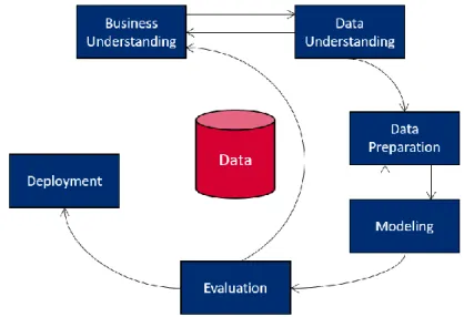
CRISP-DM provides a structured approach together with guidelines to help an individual execute a data mining project. The CRISP-DM methodology has an iterative nature and consists of six key phases (Pete Chapman et al. 2000):

1. Business Understanding – uncover important factors including success criteria, business and data mining objectives and requirements as well as business terminologies and technical terms.

2. Data Understanding – data collection, checking data quality and exploring the data to get insight of data to form hypotheses.

(15)

5 3. Data Preparation – selection and preparation of the final data set. Includes tasks such as,

data cleansing, integration, transformation and variable selection.

4. Modeling – selection and application of various data mining models and algorithms.

5. Evaluation – interpretation of the models and algorithms used and evaluating whether they achieve the objectives properly or not.

6. Deployment – determining the use the obtained results have by organizing, reporting and presenting the gained knowledge when and where needed.

Figure 1 – CRISP-DM architecture

Source: Made by the author, adapted from (Pete Chapman et al. 2000)

2.2. S

PORTS

A

NALYTICS

Sports and analytics have always had a close relation as in most sports both players and teams are measured by some form of statistics, which are used to provide rankings for both players and teams. During the 20th_{century, sports started to appeal to the masses and the broadcast of sports events}

became accessible to the general audience, which led broadcasting companies to start using different statistics to offer a better experience to the audience. The increase in popularity was met with economic benefits for the sports world and researchers started using basic statistics to better understand the games and provide insights to the stakeholders (Albert and Koning, 2008).

2.2.1. Evolution of Sports Analytics

This chapter serves as a bridge which will connect the surge of sports statistics in the mid-20th

century to the present. The main driver of this portion will be the identification and understanding of the main studies and events that led to the present concept of sports analytics.

In 1968, Charles Reep was the first data analyst connected to football and developed the base for football notation, which helps categorize each play in a match. Together with the statistician Bernard Benjamin, he looked for insights in 15 years’ worth of matches using his notation. The study helped the development of football tactics, suggesting that a more direct style of football would be desirable (Reep & Benjamin, 1968).

(16)

6 In 1977, Bill James was one of the pioneers in the application of statistics to several aspects of baseball. He defied traditional perceptions on how to evaluate players and highlighted the importance of creating runs versus basic statistics like hitting average and earned run average. His ideas captivated a lot of interest and he wrote numerous editions of The Baseball Abstract3_{where he}

presents advanced statistics and methods that are now considered the foundations for modern sabermetrics4_{(James, 2001).}

During the 1980’s, Dean Oliver inspired by Bill James sabermetrics began developing analysis on basketball players performance and their contribution to the team. His research and commitment originated what is now known as APBRmetrics5_{. Due to his great developments and achievements, in}

2004 he was hired as the first full-time statistical analyst in the NBA (Oliver, 2004).

Even with the success of Reep, Benjamin, Oliver and James sports analytics never settled inside sports organizations until the recent event commonly known as Moneyball. Billy Beane and Peter Brand used several sabermetrics and other analytics tools to create a roster of players which were considerate not very good for most teams and reached the playoffs in one of the most inspiring seasons in MLB history (Lewis, 2004). This event was for most the turning point for the use of analytics in sports.

A recent example of sports analytics taking a team to the next level is the history of the Houston Astros road to win over the Los Angeles Dodgers in the 2017 World Series6_{. The Houston Astros had}

consecutive losing records from 2011 to 2014 where they traded away their star players and veterans for future benefits, also known as tanking7_{, which with the use of a data driven mentally led}

them to the top of Major League Baseball (Sheinin, 2017).

2.2.2. Data Mining in Sports

Recently, the sports industry is experiencing a growth in terms of data mining models which search for a deeper understanding regarding various aspects of in field and off the field events. These models are being built for a multitude of sports and cover different parts of the game, player’s performance and other factors that may affect the outcome of the game (Albert and Koning, 2008). Most models attempt to predict future events in the sports world, whether for performance or gambling. For example, Edelmann-Nusser, Hohmann and Henneberg (2002) tried to predict the competitive performance of a swimmer at the Summer Olympics Games in 2002 using an artificial neural network. Another example would be the application of decision trees for identifying characteristics in matchups between players and their interactions which drive the result of hockey games (Morgan, Williams & Barnes, 2013). Finally, another popular use of predictive modeling is the forecast of the NCAA men’s basketball playoffs, which attracts multiple people to Kaggle contests and fantasy sports websites. In 2015, Yuan et al. present a famous mixture of modelers approach to try and forecast the 2014 version of these playoffs.

3_{http://baseballanalysts.com/archives/2004/07/abstracts_from_12.php} 4_{http://sabr.org/sabermetrics}

5_{http://www.apbr.org}

6_{The World Series is the annual championship series of Major League Baseball (MLB) in North America} 7_{In sports, tanking is the mentality of selling/losing present assets to achieve greater benefits in the}

(17)

7 A major factor in understanding how important sports analytics is for a sport and in what areas it is most useful is luck. Mauboussin (2012) tries to calculate the amount of luck present in several sports by giving the assumption that the observed variance in the win-lost record of a regular season is given by the variance of the skill plus the variance of luck for the given sport. In the end of a season it Is known the observer variance and, by simulating the entire season with the results at random he calculates the variance of luck:

Equation 2: Probability of winning MLB beat the streak Source: Made by the author, adapted from (Mauboussin, M., 2012) Finally, he tested the following games over 5 seasons and achieved the following results:

Figure 2: Luck in sports

Source: Made by the author, adapted from (Mauboussin, M., 2012)

According to Mauboussin (2012) these results reflect several aspects of the sports. For example, sports where there are more players in play are harder to predict than sports than sports where a small number of players influence the outcome of the game. Other important factors mentioned are the number of the regular season games, the number of opportunities per game and the type of events that form the game. The latter aspect means that a sport with more discrete events, like baseball, is easier to demonstrate the skill of players than a more fluid type game like hockey. Finally, sports that are bound by other external factors, such as meteorological, altitude or even the distance a team needs to travel to play the game tend to steer to the luck side of the diagram.

Analyzing baseball through this perspective there are mix of the above-mentioned factors that put it around the middle of the diagram. Factors like the number of games are not particularly important for the approach used in this paper since the objective is to understand bases hits instead of season wins. Nevertheless, it is quite interesting that baseball events are among the most discrete in sports, there are not a lot of participants in each event (usually only the batter, the pitcher and one or two fielders) and the number of opportunities to score are arguably high. Even considering the above-mentioned characteristics baseball is still quite random when it comes to base hits and it is crucial to interpret every possible variable, both external and internal, to better predict these outcomes (Bailey, S., 2017).

2.3. B

ASEBALL

A

NALYTICS

The use of analytics in baseball is nowadays a common practice and a lot of historical baseball data is publicly available. According to a study carried by Morton Intelligence (2018) there are more MLB organizations using analytics than in any other major league in North America.

(18)

8 Figure 3: Percentage of Sports organizations that use analytics, in North American Major Leagues

Source: Made by the author, adapted from (Mordor Intelligence, 2018)

2.3.1. State of Data Mining in Baseball

Nowadays, most baseball studies using data mining tools focus on the financial aspects and profitability of the game (Sykora, Chung, Folland, Halkon, & Edirisinghe, 2015). The understanding of baseball in game events is often relegated to sabermetrics: “the science of learning about baseball through objective evidence” (Wolf, 2015). Most sabermetrics studies concentrate in understanding the value of an individual and once again are mainly used for commercial and organizational purposes (Ockerman & Nabity, 2014; Robinson, 2014). The reason behind the emphasis on the commercial side of the sport is that “it is a general agreement that predicting game outcomes is one of the most difficult problems on this field” (Valero, C., 2016) and operating data mining projects with good results often requires investments that demand financial return.

Apart from the financial aspects of the game, predictive modelling is often used to try and predict the outcome of matches (which team wins a game or the number of wins a team achieves in a season) and predicting player’s performance. The popularity of this practice grew due to the expansion of sports betting all around the world (Stekler, Sendor, & Verlander, 2010). The results of these models are often compared with the Las Vegas betting predictions, which are used as benchmarks for performance. Projects like these are used to increase ones earning in betting but could additionally bring insights regarding various aspects of the game. (Jia, Wong & Zeng, 2013; Valero, C., 2016). In conclusion, a big reason baseball models do not reach greater predictive results is due to luck. This concept is explored by Albert (2015) and Albert (2016) where the author creates methods for predicting player’s batting average where he emphasizes that around half of the variability of a player batting average can be attributed to luck. In other words, there are several aspects of the game that are hard to translate into data and result in a higher unpredictability in these types of events. Hence the real objective of any data mining model of this type should be to minimize the effect of luck in the model (Bailey, 2017).

(19)

9

2.3.2. Statcast

Statcast is a relatively new data source that was implemented in 2015 across all MLB parks. According to MLB.com Glossary (MLB, 2018b) “Statcast is a state-of-the-art tracking technology that allows for the collection and analysis of a massive amount of baseball data, in ways that were never possible in the past. (…) Statcast is a combination of two different tracking systems -- a Trackman Doppler radar and high definition Chyron Hego cameras. The radar, installed in each ballpark in an elevated position behind home plate, is responsible for tracking everything related to the baseball at 20,000 frames per second. This radar captures pitch speed, spin rate, pitch movement, exit velocity, launch angle, batted ball distance, arm strength, and more.”

Prior to Statcast the public had access to data through PITCHf/x, which measured several parameters, including pitch speed, trajectory speed and release point. PITCHf/x was created by Sportvision and was implemented since 2008 in every MLB stadium (Fast, 2010). The video monitoring, provided by Statcast, provides the public access to a wider range of variables, player and ball tracking which is a great breakthrough for both baseball analysts and baseball in general.

(Albert, et al., 2018) developed an independent report using Statcast data to analyze possible causes for the recent surge in Home Runs in the MLB. They used variables such as the launch angle, exit velocity and many others and reached the conclusion that this increase was primarily related to a reduction in drag of the baseballs. This is a great showing of the potential of Statcast and that it is rapidly surpassing the previous methods, like PITCHf/x and could consequently lead to more precise measurements of player’s abilities (Sievert & Mills, 2016).

2.3.3. Beat the Streak

The MLB Beat the Streak is a betting game based on the commonly used term hot streak, which in baseball is applied for players that have been performing well in recent games or that have achieved base hits on multiple consecutive games. The objective of the game is to pick 57 times correctly in a row a batter that achieves a base hit on the day that it was picked. The game is called Beat the Streak since the longest hit streak achieved was 56 by the hall of famer Joe DiMaggio, during the 1941 season. The winner of the contest, which in run annually wins US$ 5.600.000, with other prizes being distributed every time a better reaches a multiple of 5 in is streak, for example picking 10 times or 25 times in a row correctly (Beat the Streak, 2018).

Some relevant rules that are important for the strategy of reaching higher streaks are: the better can select 1 or 2 batters per day but note that the streak does not end if no batter is picked for a given day. If the player selected does not start the game for any reason the player is not accounted as an actual pick. Nevertheless, if the player is switched mid game without achieving a base hit, the streak is reset. Finally, there is a Mulligan which works as a second change for when the streak of a better lies between 10 and 15. If the better incorrectly picks during this state of his streak, his streak will remain (Beat the Streak, 2018).

To better visualize the different rules, table 1 illustrates some examples on how the streak works in different scenarios:

(20)

10 Pick 1 Pick 2

Hit Hit Not Hit Not Hit

Hit Not Hit Pass Not Hit Hit Pass Pass Pass

Result

Streak is preserved at the current level Streak is increased by one (1)

Streak ends and resets to zero unless a Mulligan applies in which case the streak is preserved at the current level Streak ends and resets to zero unless a Mulligan applies in which case the streak is preserved at the current level Streak ends and resets to zero unless a Mulligan applies in which case the streak is preserved at the current level Streak increases by two (2)

Table 1: Beat the Streak scenario outcomes

Source: Made by the author, adapted from (Beat the Streak, 2018)

2.3.4. Predicting batting performance

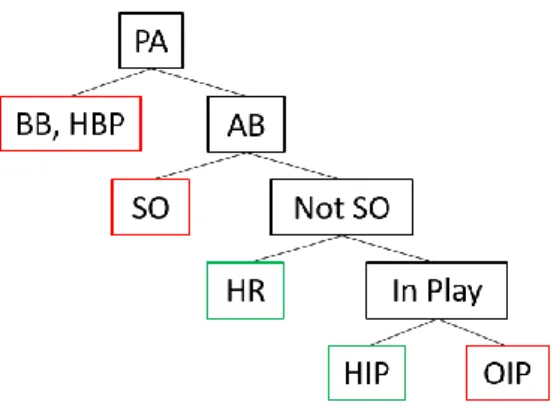
Baseball is a game played by two teams who take turns batting (offense) and fielding (defense). The objective of the offense is to bat the ball in play and score runs by running the bases, whilst the defense tries to prevent the offense from scoring runs. The game proceeds with a player on the fielding team as the pitcher, throwing a ball which the player on the batting team tries to hit with a bat. When a player completes his turn batting he gets credited with a plate appearance, which can have one of the following outcomes, as seen below:

Figure 4: Breakdown of a plate appearance Source: Made by the author, adapted from (Albert, 2015)

Denotated in green are the events which result on a base hit and in red the events which are not. Thereafter, what this paper tries to achieve is to predict if a batter will achieve a Home Run (HR) or a Ball hit in play (HIP) among all his plate appearances during a game. The most common approach which mostly resembles the model built in this project is forecasting the batting average (AVG). The differences from both approaches are that the batting average does not account for Base on Balls (BB) and Hit by Pitches (HBP) scenarios.

Equation 3: Batting Average and Hitting Percentage calculation Source: Made by the author

(21)

11 There are many systems which predict offensive player performance including batting averages. These models range from simple to complex. Henry Druschel from Beyond the Boxscore identifies that the main systems in place are: Marcel8_{, PECOTA}9_{, Steamer}10_{, and ZiPS}11_{(Druschel ,2016; Bailey,}

2017).

• Marcel encompasses data from the last three seasons and gives extra weight to the most recent seasons. Then it shrinks a player’s prediction to the league average adjusted to the age using a regression towards the mean. The values used for this are usually arbitrary. • PECOTA uses data for each player using their past performances, with more recent years

weighted more heavily. PECOTA then uses this baseline along with the player's body type, position, and age, to identify various comparison players. Using an algorithm resembling k-nearest neighbors, it identifies the closest player to the projected player and the closer this comparison is the more weight that comparison player's career carries.

• Steamer uses a weighted average of past season performances adjusted to the league average. Steamer, much like Marcel, then looks to regress the prediction towards the mean but the degree and weight is regressed varies. Those are set using regression analysis of past players.

• ZiPS like Marcel and Steamer uses a weighted regression analysis but specifically four years of data for experienced players and three years for newer players or players reaching the end of their careers. It then pools players together based on similar characteristics.

Bailey, Loeppky and Swartz (2017) use PECOTA in conjunction with Statcast data to eliminate some of the effect of luck in predicting player’s batting average. The objective of the paper is to improve the performance of PECOTA using the aforementioned data. The solution is achieved by simply combining both techniques using a linear regression. The results are a very marginal improvement that prove that there are potential gains in using Statcast data and variables that come from this source.

Goodman and Frey (2013), developed a machine learning model to predict the batter most likely to get a hit each day. Their objective was to win the MLB Beat the Streak game, to do this they built a generalized linear model (GLM) based on every game since 1981. The results on testing were 70% precision on correct picks and in a real-life test achieved a 14-game streak with a peak precision of 67,78%

Clavelli and Gottsegen (2013), created a data mining model with the objective of maximizing the precision of hit predictions in baseball. The project compiles game data from previous seasons and uses a logistic regression, which achieves a 79,3% precision on its testing set. In the paper it is also used a support vector machine, which heavily overfitted and only achieved a 63% precision in its testing set.

8_{Marcel - Available at http://www.tangotiger.net/marce} 9_{PECOTA - Available at https://www.baseballprospectus.}

10_{Steamer - Available at http://steamerprojections.com/blog/about-2} 11_{ZiPS – Available at https://www.fangraphs.com}

(22)

12 Figure 5: Literature review summary

(23)

13

3. METHODOLOGY

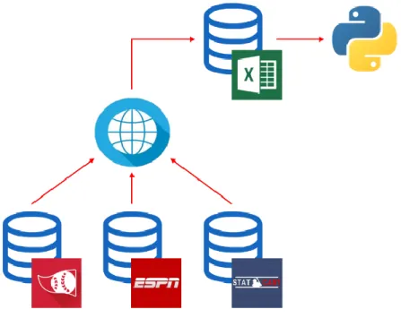
This section of the paper presents the methodological processes done from the collection and creation of the dataset until the evaluation of the final models. As explored during the literature review, the project follows the popular architecture for data mining projects CRISP-DM and, this chapter is focused on the data understanding, data preparation, modelling and evaluation processes. Figure 6 depicts the various software used to complete these tasks, which were Microsoft Excel and Python. In a first stage, Microsoft Excel was used for data collection, data integration and for variable transformation purposes. In a second stage, the dataset was imported to Python where the remaining data preparation, modeling and evaluation processes were carried out. In Python the three crucial packages used were Pandas (dataset structure and data preparation), Seaborn (data visualization) and Sklearn (for modeling and model evaluation).

Figure 6: Data sources and data management diagram Source: Made by the author

Scikit-learn is a popular Python library that has a collection of machine learning algorithms, for both supervised and unsupervised learning. Furthermore, it includes many functions and applications that enable some preprocessing, modelling and evaluation steps of a data mining project. Finally, it is known for being easy to integrate in many applications since it relies on the Python ecosystem and thus is used in wide range of subjects (Michel et al., 2011, Pedregosa et al., 2011)

Finally, figure 7 illustrates an overall view of the project, showing the process performed on each of the training sets and the main constrains that separate the final 48 models, beginning in the raw dataset and finishing in the evaluation procedures, note that the final evaluation procedures were performed for both the validation set, i.e. data partitioning the training set using a 10-fold cross validation and for the test set which was separated initially and, the only treatment perform on the latter was normalization of the variables.

(24)

14 Figure 7: Top down model creation diagram

Source: Made by the author

3.1. D

ATA

C

OLLECTION

This sub-chapter will describe which data sources were used and resumes the process that was carried out to arrive to the final dataset. The data considered for this study were the games played in Major League Baseball for the seasons 2015, 2016, 2017 and 2018.

The features were collected from the three open source websites:

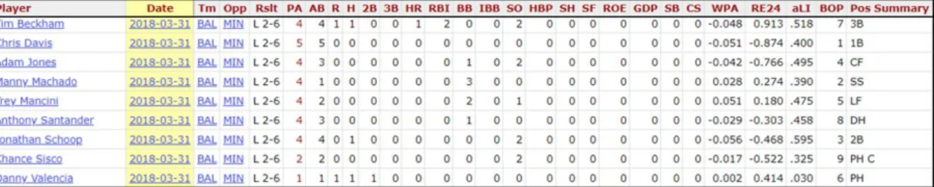
1. Baseball Reference – Baseball Reference is a subsection of the Sports Reference website; the latter includes several other sport related websites. They attempt to give a comprehensive approach to sports data. In their baseball section it is possible to find extensive information about baseballs teams, baseball players, baseball statistics and other baseball related themes dating back to 1871. The data collected from this source is game-by-game player statistics and weather conditions, which could be sub-divided into batting statistics, pitching statistics and team statistics. Data was displayed in a box-score like manner, has seen in the table 2 (Baseball Reference, 2018).

2. ESPN – ESPN is a famous North American sports broadcaster with numerous television and radio channels. ESPN mainly focus on covering North American professional and college sports such as, basketball, American football or baseball. Their website contains live scores, news, statistics and other sports related information up to date. The resource retrieved from the ESPN website was the ballpark factor (ESPN, 2018).

3. Baseball Savant – Baseball Savant provides player matchups, Statcast metrics and advanced statistics in a simple and easy-to-view way. These include several data visualization applications which help users explore Statcast data. The data retrieved from this data source

(25)

15 includes Statcast yearly player statistics, such as average launch angle, average exit velocity, etc (Baseball Savant, 2018).

Table 2: Sports Reference box-score display Source: Made by the author (Baseball Reference, 2018)

In order to build the final dataset, the different features were saved in Excel Sheets. From Baseball Reference three sub sections were created: batter scores, pitcher scores and team box-scores. From Sports Savant batter yearly Statcast statistics. From ESPN the ballpark related aspects. Note that, since the data came from different data sources there was a need to integrate the variables into a single dataset. This process was performed in Microsoft Excel, where with the help of player’s name, date or other relevant features it was created the necessary primary keys, these in conjunction with the VLOOKUP function in Microsoft Excel enabled the integration of the data. There were some records that did not coincide or that needed further work, are mentioned in the data preparation chapter.

3.2. D

ATA

U

NDERSTANDING

This sub-chapter will serve the purpose of explaining the category of the features present in the dataset, to help understanding the variables used to create the models and the transformations applied to the features. These objectives will be met with using descriptive statistics and data visualization techniques.

3.2.1. Category description

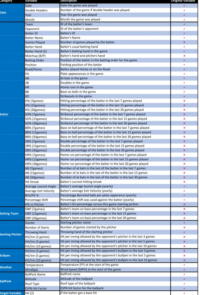
Throughout the literature review several projects and papers were analyzed and, from which we could hypothesize the best categories for this paper. Along this chapter the chosen features categories will be explained for a general understanding on what they are and their potential importance for the models. The table 3 includes a description for all the features in the final dataset.

(26)

16

Category Variable Description Original Variable

Date Date the game was played a

Double Headers Number of the game if double header was played a

Year Year the game was played a

Month Month the game was played a

Team ID of the batter's team a

Opponent ID of the batter's opponent a

Batter ID Batter's ID a

Batter Name Batter's Name a

Games Played Number of games played by the batter r

Batter Hand Batter's usual batting hand a

Batter Hand (2) Batter's batting hand in this game a

Matchup (B/P) Batter's hand and pitchers hand r

Batting Order Position of the batter in the batting order for the game a

Position Fielding position of the batter a

Road/Home Batter played Home or on the Road a

PA Plate appearances in the game a

AB At bats in the game a

2B Doubles in the game a

HR Home runs in the game a

BB Base on balls in the game a

SO Strikeouts in the game a

H% (7games) Hitting percentage of the batter in the last 7 games played r

SO% (7games) Strikeout percentage of the batter in the last 7 games played r

BB% (7games) Base on ball percentage of the batter in the last 7 games played r

2B% (7games) Double percentage of the batter in the last 7 games played r

HR% (7games) Home run percentage of the batter in the last 7 games played r

AB (7games) Number of at bats in the last of the batter in the last 7 games r

Hit Streak Batter's current hitting streak r

Average Launch Angle Batter's average launch angle (yearly) a

Average Exit Velocity Batter's average Exit Velocity (yearly) a

Brls/PA % Percentage Barreled balls per plate apperance (yearly) a

Percentage Shift Percentage shift was used against the batter (yearly) a

H% vs Pitcher Batter's hit percentage versus this game starting picther r

OBP (7games) Batter's team on base percentage in the last 7 games r

Starter Starting pitcher name a

Number of Starts Number of games started by the pitcher r

Throwing Hand Throwing hand of the starting pitcher a

Hit/Inn (3 games) Hit per inning allowed by the opponent's pitcher in the last 3 games r

Hit/Inn (3 games) Hit per inning allowed by the opponent's bullpen in the last 3 games r

Temperature Temperature (Fº) at the start of the game a

WindSpd Wind Speed (MPH) at the start of the game a

BallPark Name BallPark name a

Altitude Altitude of the ballpark a

Roof Type Roof type of the ballpark a

ESPN Hit Factor ESPN hit factor for the ballpark a

Target Variable Hit (2) If the batter got a base hit a

Weather BallPark Date Batter Batting Team Starting Pitcher Bullpen

Table 3: Variable description Source: Made by the author

(27)

17

A. Batter’s performance

These variables look to describe characteristics, conditions or the performance of the batter. These variables translate into data features like the short/long term performance of the batter, tendencies that might prove beneficial to achieve base hits or even if the hand matchup, between the batter and pitcher, is favorable. The reason behind the creation of this category is that selecting good players based on their raw skills is a worthwhile advantage for the model.

B. Batter’s team performance

The only aspect that fits this category is the on base percentage (OBP) relative to the team’s batter. Since baseball offense is constituted by a 9-player rotation if the batter’s team mates perform well, i.e. get on base, this leads to more opportunities for the batter and consequently higher number of at-bats to get a base hit.

C. Opponent starting pitcher’s performance

The variables in this category refer to recent performance of the starting pitcher. These variables relate to the pitcher’s performance in the last 3 to 10 games and the number of games played by the starting pitcher. The logic behind the category is that the starting pitcher has a big impact on preventing base hits and the best pitchers tend to allow fewer base hits than weaker ones.

D. Opponent bullpen’s performance

This category is quite similar to the previous one. Whereas the former category looks to understand the performance of the starting pitchers the latter focus on the performance of the bullpen, i.e. the remaining pitchers that might enter the game when starting pitcher get injured, get tired or enter to create tactical advantages. The reasoning for this category is exactly the same as the previous one, a weaker bullpen tends to provide a higher change of base hits than a good one.

E. Weather Conditions

In terms on weather conditions, the features that are taken into account are wind speed and temperature. Firstly, the temperature affects a baseball game in 3 main aspects: the baseball physical composition, the player’s reactions and movements, and the baseball’s flight distance (Koch & Panorska, 2013). If all other aspects remain constant higher temperatures lead to a higher chance of offensive production and thus base hits. Secondly, wind speed affects the trajectory of the baseball, which can lead to lower predictability of the ball’s movement and even the amount of time a baseball spends in the air (Chambers, Page & Zaidinis, 2003).

F. Ballpark

Finally, ballpark englobes the ESPN ballpark hit factor, the roof type and the altitude. The “Park factor compares the rate of stats at home vs. the rate of stats on the road. A rate higher than 1.000 favors the hitters. Below favors the pitcher” meaning that this factor will have into consideration several aspects from this or other categories, indirectly (ESPN, 2018). Altitude is another aspect that is crucial to the ballpark, the higher the altitude the ballpark is situated the farther the baseball tends to travel. The previous statement is important to the Denver’s Coors Field, widely known for its unusually high offensive production (Kraft & Skeeter, 1995). Finally, the roof type of the ballpark

(28)

18 affects some meteorological metrics, since a closed roof leads to no wind and a more stable temperature, humidity, etc when compared to ballparks with and open roof.

3.2.2. Data Exploration

This chapter serves the purpose of understanding data in a deeper level. Using descriptive statistics and visualization techniques it will be possible to identify certain aspects of the dataset that enable other preprocessing steps, making them more accurate and easier to comprehend.

It should be noted that some of the variables in the dataset were only used for the construction of said dataset and, thus were not explored using the methods mentioned above. Therefore, the variables represented in this chapter are the ones that were taken into consideration for modelling purposes.

3.2.2.1. Descriptive Statistics

Regarding the descriptive statistical analysis of the variables, the results are shown in table 4 for the numeric variables and in table 5 for the nominal variables. For the numerical variables it is possible to access the mean, standard deviation, variance, min-max and the minimum and maximum standard deviation, per feature. The tables enable the understanding of the variables at a univariate level and these values will be particularly useful for outlier detection process.

For the categorical values it is represented the number of levels and the mode. These statistics were crucial for variable selection regarding algorithms which cannot handle categorical variables and thus needed some sort of transformation. In sum, variables with a lot of levels are harder to adapt to numeric values if they do not have an order of magnitude and, in these cases are less likely to be picked due to these constrains.

Finally, it was calculated the Pearson’s and Spearman’s correlation with the objective of uncovering relationships between the independent and with the dependent (target) variable. According to Larose (2005), the former is helpful for not overemphasizing one data component, i.e. using correlated variables might cause the models to become unstable and deliver unreliable results. In contrast, the latter is used for finding features that have a higher predictive power. Therefore, avoid choosing variables that are highly correlated between one another and take special attention to variables that are highly correlated to the target variable.

Pearson’s correlation was first described in 1896 and according to Hauke and Kossowski (2011) is” a measure of strength of the relationship between two variables that cannot be measured quantitatively”. The main disadvantage of the Pearson’s correlation is that it assumes a normal distribution of the features and thrives at finding linear relationships in the data.

With these constrains in mind soon emerged another form of evaluating correlation between features. The Spearman’s rank correlation is nonparametric, i.e. does not make assumptions on the distribution of the data and can find nonlinear relationships between the features (Hauke & Kossowki, 2011).

Nevertheless, none of the two is perfect and thus by calculating both types of correlations it will be possible to achieve a better understanding of the relationships between the features and in conclusion make the best use of the data.

(29)

19

Category Variable Unit Average Std. Dev. Variance Minimum Maximum Min Std.Dev. Max. Std.Dev. Distribution

Batter Game Number of Games 182,85 142,53 20.313,69 2,00 634,00 -1,27 3,17

Batting Order 1 - 9 4,72 2,46 6,04 1,00 9,00 -1,51 1,74 H% (7games) % 0,23 0,08 0,01 0,00 1,00 -2,80 9,25 H% (15games) % 0,23 0,06 0,00 0,00 1,00 -3,80 12,51 H% (30games) % 0,23 0,05 0,00 0,00 1,00 -4,72 15,49 SO% (7games) % 0,21 0,10 0,01 0,00 1,00 -2,12 8,20 SO% (15games) % 0,21 0,08 0,01 0,00 1,00 -2,56 9,89 SO% (30games) % 0,20 0,07 0,01 0,00 1,00 -2,83 10,98 BB% (7games) % 0,16 0,08 0,01 0,00 0,80 -1,93 7,81 BB% (15games) % 0,16 0,06 0,00 0,00 0,80 -2,80 11,25 BB% (30games) % 0,16 0,05 0,00 0,00 0,80 -3,52 14,13 2B% (7games) % 0,05 0,04 0,00 0,00 0,75 -1,13 17,23 2B% (15games) % 0,05 0,03 0,00 0,00 0,75 -1,56 23,68 2B% (30games) % 0,05 0,02 0,00 0,00 0,75 -1,97 29,80 HR% (7games) % 0,03 0,04 0,00 0,00 0,40 -0,87 10,21 HR% (15games) % 0,03 0,03 0,00 0,00 0,40 -1,15 13,42 HR% (30games) % 0,03 0,02 0,00 0,00 0,40 -1,38 16,06 AB (7games) At Bats 25,89 3,65 13,29 1,00 39,00 -6,83 3,60 AB (15games) At Bats 54,47 9,23 85,13 1,00 76,00 -5,80 2,33 AB (30games) At Bats 105,25 23,99 575,37 1,00 144,00 -4,35 1,62

Hit Streak Number of Games 1,97 2,49 6,21 0,00 30,00 -0,79 11,25

Average Launch Angle Launch Angle (º) 11,57 4,62 21,37 -35,70 41,70 -10,23 6,52

Average Exit Velocity Miles per Hour (MPH) 88,09 3,67 13,45 58,60 115,70 -8,04 7,53

Brls/PA % % 0,05 0,03 0,00 0,00 0,40 -1,67 12,22

Percentage Shift % 0,15 0,21 0,04 0,00 0,94 -0,72 3,83

H% vs Pitcher % 0,23 0,17 0,00 0,00 1,00 -1,40 4,58

(30)

20

Category Variable Unit Average Std. Dev. Variance Minimum Maximum Min Std.Dev. Max. Std.Dev. Distribution

OBP (7games) % 0,32 0,03 0,00 0,20 0,44 -3,54 3,44

OBP (15games) % 0,32 0,02 0,00 0,22 0,43 -3,94 4,67

OBP (30games) % 0,32 0,02 0,00 0,22 0,43 -5,12 6,05

Starting Pitcher Game Number of Games 37,91 29,43 866,39 2,00 131,00 -1,22 3,16

Hit/Inn (3 games) Hits per Inning 1,04 0,41 0,17 0,00 30,00 -2,56 71,02

Temperature Fahrenheit (Fº) 73,70 10,56 111,48 27,00 108,00 -4,42 3,25

WindSpd Miles per Hour (MPH) 7,49 5,04 25,40 0,00 28,00 -1,49 4,07

Altitude Feet (ft) 504,80 917,08 841.036,27 0,00 5.197,00 -0,55 5,12

ESPN Hit Factor - 1,00 0,08 0,01 0,84 1,30 -1,98 3,65

Batting Team

Starting Pitcher

Bullpen

Weather

Ballpark

Table 4: Descriptive statistics for numeric variables Source: Made by the author

Category Variable Type N. Levels Mode Occurance percentage per label

Matchup (B/P) Categorical 4 R/R R/R = 37%; L/R = 35%; R/L = 22%; L/L = 6% Road/Home Binary 2 Away Away = 50%; Home = 50%

Batter Hand (2) Binary 2 Right Right = 59%; Left = 41%

Starting Pitcher Throwing Hand Binary 2 Right Right = 72%; Left = 28%

Ballpark Roof Type Categorical 3 Open Open = 77%; Retractable = 20%; Fixed = 3%

Target Variable Hit (2) Binary 2 Yes Yes = 65%; No = 35%

Batter

Table 5: Descriptive statistics for categorical variables Source: Made by the author

3.2.2.2. Data Visualization

Data visualization is a focal point of any data related word. The concept was popularized by John Tukey (1961) where he defines data analysis as the “procedures for analyzing data, techniques for interpreting the results of such procedures, ways of planning the gathering of data to make its analysis easier, more precise or more accurate, and all the machinery and results of (mathematical) statistics which apply to analyzing data”.

In the context of the paper, the best approach was to use both univariate and bivariate visualization techniques. Several types of plots were designed to not only understand the data, but more

(31)

21 importantly to provide a good perception of the facts hidden in the dataset without needing a lot knowledge on the topic of baseball.

Firstly, as seen in table 4, all numeric variables distribution plots were analyzed, these graphs greatly complement other visualization techniques as, for example, it gives a first impression on outliers and their magnitude. Additionally, the distribution plot provides a perception on the distributions of the features, which is essential if further statistical testing is required.

Continuing the topic of outlier detection, boxplots were used to test for outliers in all numeric values. This topic is further explored in the data preparation chapter, where these plots are used in conjunction with some of the descriptive statistics shown previously to detect extreme values that need to be dealt with.

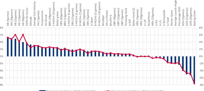
As mentioned in the previous subchapter, data correlation will be of great importance in more than a few processes of the paper. Therefore, in figure 8 are plotted the Pearson’s and the Spearman’s correlation between the dependent features and the independent features. The correlation values between dependent variables were also calculated, but due to their extensive nature can be found in annexes 8.3 and 8.4. A B ( 7g a me s) H % ( 3 0g ame s) A B ( 15 ga me s) H % ( 1 5g ame s) A B ( 30 ga me s) ES P N H it Fa cto r A lti tu de A ve ra ge E xi t V e lo ci ty H % ( 7 ga me s) Te mp er a tu re H it Str e ak B B % ( 3 0g ame s) S H it/ In n (1 0 g ame s) B att e r g ame 2 B % ( 3 0 ga me s) B B % ( 1 5g ame s) S H it/ In n (5 g a me s) 2 B % ( 1 5 ga me s) S H it/ In n (3 g a me s) B H it/ In n ( 3 ga me s) B B % ( 7 ga me s) 2 B % ( 7 ga me s) Is Op en B H it/ In n ( 5 ga me s) B H it/ In n ( 10 g ame s) W in d Sp d H % v s P itc h er B rl s/ P A % O B P ( 30 ga me s) O B P ( 15 ga me s) O B P ( 7g a me s) Th ro w in g H an d Is R /R B att e r H an d ( 2) H R % ( 7 ga me s) H R % ( 3 0g a me s) Is L /R R o ad /H o me H R % ( 1 5g a me s) Is R /L Is L /L Is R e tr ac ta b le Is F ix ed P itc he r G ame A ve ra ge L au n ch A n gl e P er ce n ta ge S h if t SO% (7 ga me s) SO% (1 5 ga me s) SO% (3 0 ga me s) B att in g Or d e r -8% -6% -4% -2% 0% 2% 4% 6% 8% -8% -6% -4% -2% 0% 2% 4% 6% 8%

Pearson's correlation with Target Variable Spearman's correlation with Target Variable

Figure 8: Pearson’s and Spearman’s correlation for target variable Source: Made by the author

As seen in the correlation plot, there is no variable with a huge correlation to the target variable but batting order, number of at-bats in previous games and mostly other batter performance variables look to have the most impact on the target variable, at first sight. Nonetheless, these values are very insightful, and it is feasible to select some of top variable, to explore visually.

(32)

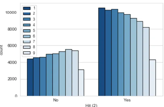
22 Figure 9: Batting order influence on base hits

Source: Made by the author

Figure 9 depicts the relation between the batting order and if the batter got a base hit in the game. The graph shown matches the negative correlation value of this pair of variables, where the batters in the first positions of the lineup are considerably more likely to get base hit than the bottom of the lineup. This result is a consequence of the fact that the top of lineup bats more often that the bottom of the lineup, thus coaches use these spots for the most talented batters of the team, which usually have the best results. Note that the gap seen in the 9th_{position is mostly the consequence of}

removing pitchers batting from the dataset, since very often they bat last in the lineup.

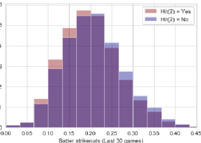
Figure 10: Number of games played by the batter influence on base hits Source: Made by the author

Another variable taken into consideration when factoring batter performance was the number of games a batter has played. This translates into how experienced a batter is and, as seen in the graph above, there are some insights that are not completely linear. Briefly, a batter with very few games played does not have much success in term of base hits, similarly like batters with a lot of games under their belt. In terms of this feature, there looks to exist a sweet spot or what is commonly known as the prime years of an athlete.

The main factors that affect players of their carrer in baseball are, according to Staszewski & Siegler (1994), physical development which usually peaks at 28-30 years of age, experience which constantly grows during a player’s carrer and wear and tear which negatively impacts the player’s performance and over the years make a player’s more susceptile to injury and to lose of overall performance.