Biogeochemical modelling of the NW Iberian Margin

      Universidade de Aveiro 2011 Departamento de Física

Carlos Rafael Vieira

Rocha

Modelação Biogeoquímica da Margem NW

Ibérica

Biogeochemical Modelling of the NW

Iberian Margin

Dissertação apresentada à Universidade de Aveiro para cumprimento dos requisitos necessários à obtenção do grau de Mestre em Meteorologia e Oceanografia Física, realizada sob a orientação científica do Prof. Dr. Jesús Manuel Pedreira Dubert, Professor Auxiliar do Departamento de Física da Universidade de Aveiro e da Dra. Maria Rita Teixeira de Sampaio Nolasco, Investigadora Auxiliar do CESAM.

Este trabalho foi desenvolvido no âmbito do projecto RAIA – “Observatório Oceânico da Margem Ibérica” (BI/0313_RAIA_1_E/UA1), co-financiado pelo Programa de Cooperação Transfronteiriça Espanha-Portugal, POCTEP, e por fundos FEDER.

o júri

presidente Prof. Doutor José Manuel Henriques Castanheira

Professor Auxiliar da Universidade de Aveiro

Doutor Paulo Nogueira Brás de Oliveira

Investigador Auxiliar do IPIMAR

Prof. Doutor Jesús Manuel Pedreira Dubert

Professor Auxiliar da Universidade de Aveiro

Doutora Maria Rita Teixeira de Sampaio Nolasco

acknowledgements I would now like to thank the help and support of the many people that contributed to the birth of this thesis.

To both my supervisors,

Prof. Dr. Jesús Dubert, for his scientific supervision, invaluable advices, great motivational talks, and for giving me the opportunity of starting my scientific career with a such an interesting project, studying a subject I everyday grow more fond of;

Dr. Rita Nolasco, my “lab supervisor”, for the great suggestions, her endless patience and will to help and for her sympathy and all-time availability in the never-ending fight against doubts and mistakes.

To MSc Nuno Cordeiro, for the unconditional and invaluable support with most of the statistics and images presented in this thesis.

To PhD student Rosa Reboreda, for walking a part of the biogeochemical modelling path with me, from our first introductory steps in its world, to more complex questions, always with a cheerful exchange of knowledge and help. To Dr. Martinho Marta-Almeida, for the instructive introductory classes to ROMS and related subjects, useful help in solving different problems, and enlightening talks.

To all others from “NEPTUNO”, the regional ocean modelling group: Dr. João Lencart e Silva, Dr. Fabiola Amorim, PhD student Ana Pires and PhD student César Ribeiro for the occasional advice or help.

To my friends, they know who they are, for all the free-time moments that make this life even more worthwhile and that are like a fuel for surpassing obstacles and hard times.

And last, but not least, to my parents, for a life-long support and presence, and the unbreakable will to help me in any way they can.

palavras-chave Ciclos Biogeoquímicos; Modelação Numérica; ROMS; Margem Ibérica.

resumo A capacidade de fornecer dados oceanográficos sobre variáveis biológicas e químicas tem-se tornado num tema de relevância científica nos últimos anos. A procura por este tipo de informação provém de áreas e aplicações tão diversas como a investigação em ecossistemas marinhos, a monitorização da qualidade da água e o suporte à gestão do ambiente marinho e costeiro. Este trabalho consiste numa visão geral sobre a incorporação de um módulo biogeoquímico baseado em fluxos de azoto (NPZD) num modelo de circulação oceânica regional (ROMS) para a Margem NW Ibérica e para o período de 2007 a 2010. O estudo foca-se especialmente na validação do modelo, tanto empírica como objectiva, através da comparação entre os valores de clorofila-a simulados e os que constam numa extensa base de dados produzida pelo Ifremer/CERSAT, assim como na verificação da capacidade de reprodução de alguns fenómenos teoricamente expectáveis. A validação do modelo mostra que, embora existam algumas falhas, como uma subestimação geral dos valores superficiais de clorofila-a ou a antecipação ao início dos blooms primaveris, a resposta deste é satisfatória. Embora ainda exista muito a melhorar, é possível afirmar que está criado um modelo com acoplamento biogeoquímica-hidrodinâmica, completamente funcional e credível, com capacidade de simulação a uma escala inter-anual para a Margem NW Ibérica.

keywords Biogeochemical Cycles; Numerical Modelling; ROMS; Iberian Margin.

abstract Providing oceanographic data on biological and chemical variables has become an issue of scientific concern over the last years. The demand for this kind of information arises from a range of fields and applications such as scientific research on marine ecosystems, monitoring of seawater quality and decision-making support for marine and coastal management. This work consists of an overview on the incorporation of a nitrogen-based (NPZD) biogeochemical module into a regional oceanic circulation model (ROMS) for the NW Iberian Margin for the 2007 to 2010 period. The study focuses especially in both empirical and objective model performance assessments through comparison of chlorophyll-a model outputs with an extensive satellite dataset produced by Ifremer/CERSAT and in the verification of the model ability to reproduce theoretically expected phenomena. The model validation shows that despite some flaws, as a general underestimation of chlorophyll-a surface values and an anticipation in the starting of the spring bloom, the model response is satisfactory. With still much to improve, its however possible to state that a fully-functional and reliable coupled biogeochemical-ocean circulation model is available for the NW Iberian Margin, running at the inter-annual scale.

CONTENTS

LIST OF FIGURES ... i

1.

INTRODUCTION ... 1

2.

STATE OF THE ART ... 3

3.

NUMERICAL OCEAN MODEL ... 5

3.1.  Brief description ... 5  3.2.  Configuration... 6  a.  First Domain ... 7  b.  Large Domain ... 7 

4.

STUDY AREA ... 9

5.

SATELLITE DATA ... 10

6.

RESULTS ... 12

7.

DISCUSSION ... 31

8.

CONCLUSIONS ... 33

9.

REFERENCES ... 34

10.

ATTACHMENTS ... 39

List of figures

i

LIST OF FIGURES

Figure 1 – Scheme illustrating the basic scales of organisms and ocean characteristics of

importance to the theme in discussion (Mann et al., 2006)... 3

Figure 2 – Schematic representation of the NPZD model processes... 5

Figure 3 – Illustration of the “First Domain” (FD - on the left) and “Large Domain” (LD - on the right) geographic localization with identification of the main bathymetric lines. The study area (adressed in its own chapter) is also represented... 6

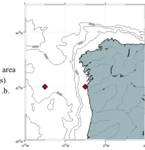
Figure 4 – Geographical localization of the study area with identification of the main isobaths (in meters) and the location of the grid boxes featuring in 6.1.b... 9

Figure 5 – Chlorophyll-a map for 13 of February 2008. Units are in milligrams of chlorophyll-a per cubic meter (adapted from ftp://ftp.ifremer.fr/)... 10

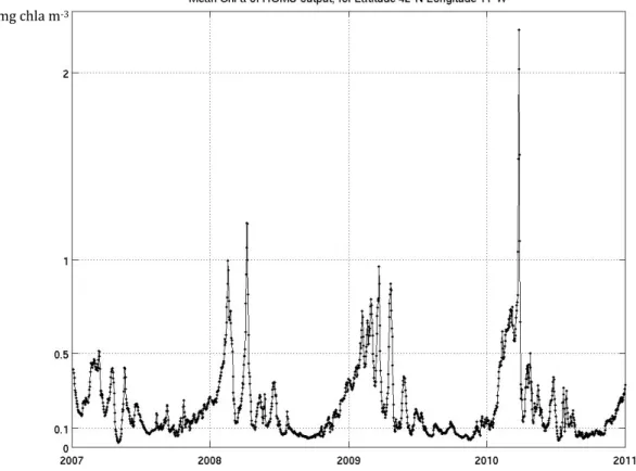
Figure 6 – Area averaged surface chlorophyll concentration (daily model output) time series for the four simulated years. The units are in milligrams of chlorophyll-a per cubic meter... 12

Figure 7 – Mean surface chlorophyll concentration (model output) time series for the four simulated years in a box of 5x5 grid points centered at 42ºN 9ºW. The units are in milligrams of chlorophyll-a per cubic meter... 13

Figure 8 – Same as Figure 7 but with the box centered at 42ºN 11ºW... 14

Figure 9 – Monthly means of chlorophyll-a for 2007-20010 period. The images are presented in seasonal groups, with model means above and satellite means below. The logarithmic colorbar presents milligrams of chlorophyll-a per cubic meter as units... 16

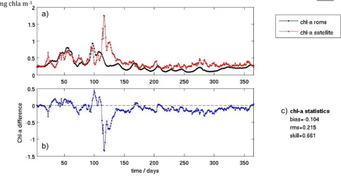
Figure 10 – (a) - 2007 area averaged surface chlorophyll concentration time series for model outputs (in black) and satellite data (in red). The units are in milligrams of chlorophyll-a per cubic meter. (b) - Direct difference between the two time series of (a). (c) - Chlorophyll-a model statistics with satellite data as reference: bias (in mg chla m-3_{), rms (in mg chla m}-3_{) and skill... 18}

Figure 11 – Same as Figure 13 for the year 2010... 19

Figure 12 – Same as Figure 13 for the year 2010... 19

Figure 13 – Same as Figure 13 for the year 2010... 20

Figure 14 – (a) Model daily outputs percentage model bias for the 2007-2010 period with satellite daily data as reference (b) Cross-correlation coefficient between model and satellite daily data for the 2007-2010 period... 21

Figure 15 – Model and satellite EOF results for 2007-2010 period. Representation of the first temporal mode (blue line for model, red line for satellite) and correspondent spatial modes (model on the left and satellite on the right)... 23

Figure 16 – Same as Figure 18 for the fourth EOF mode... 23

List of figures

ii

Figure 18 – Same as Figure 18 for the fourth EOF mode... 24 Figure 19 – Surface daily averaged values of temperature (on the left) and chlorophyll-a (on the right) for September 12, 2007. The images in the first row correspond to model outputs and the ones below to remote sensing data... 26 Figure 20 – Bloom occurrence for April 22, 2009. Illustration of surface daily averaged values of temperature (on the left) and chlorophyll-a (on the right) with the images in the first row corresponding to model outputs and the ones below to remote sensing data……..………... 27 Figure 21 – Upwelling occurrence for August 14, 2008. Surface daily averaged values of temperature (on the left) and chlorophyll-a (on the right) for the referred date. The images in the first row correspond to model outputs and the ones below to remote sensing data……...……….. 28 Figure 22 – Area averaged surface concentrations for the 2007-2010 period. Variables plotted include Nitrates (in blue), Phytoplankton (in green), Zooplankton (in red) and Detritus (light brown). All the variables are expressed in mMol N m-3_{. ... 29}

Figure 23 – Vertical profiles along a latitudinal section for August 9, 2010. All the variables are expressed in mMol N m-3 _{with exception to the Temperature, which is in ºC... 30}

Introduction

1. INTRODUCTION

1.1. Motivation

The quality and the management of the coastal and marine environments are particularly delicate issues in European social, economical and political agendas. However, genuine environmental concerns relating to the sea are often obfuscated and obscurely formulated because of, among other causes, the absence of a steady supply of reliable information (Pinardi and Woods, 2002).

Providing oceanographic data on biological and chemical variables has thus become an issue of concern over the last years. The demand for this kind of information arises from a range of fields and applications such as scientific research on marine ecosystems, monitoring of seawater quality and decision-making support for marine and coastal management. A recent questionnaire conducted by ICES-WGOOFE (International Council for the Exploration of the Sea, Working Group on Operational Oceanographic Products for Fisheries and Environment) showed that temperature, currents, salinity, chlorophyll standing stock and primary production were the most requested products among ocean sciences scientific community, who scored several biological parameters in the top 10 rankings of products on demand (Berx et al., 2011).

Marine ecology, as traditionally understood, is the study of marine organisms and their relationships with other organisms and with the surrounding environment (Mann et al., 2006), but instead of putting the organisms at the center of the picture, it is possible to work with marine ecosystems in which physical, chemical, and biological components are equally important in defining total system properties. This approach, in its holistic potential, may create the means to attain the much needed source of information, acting as a solid scientific basis for marine environment research and providing continuous evolving support for decision-makers.

In fact, the increasing understanding of fundamental processes over second to decadal time scales and centimeters to megameter space scales is beginning to influence the management of the ocean's living resources (Mann et al., 2006). We are seeing that year-to-year and decade-to-decade changes in the atmosphere are reflected in property changes in the near-surface ocean. The way in which these changes affect the growth and survival of different plankton species and the distribution of fish are two topics that will surely receive a great deal of attention in the near future.

It is important to bear in mind that the physical factors leading to fertile and infertile areas are very different on land than in the ocean, as the nutrients required by land plants are generated nearby from decaying remains of previous generations, but decaying matter in the ocean tends to sink and leave the sunlit euphotic layer where phytoplankton - main agent of primary production - grows. The nutrients are thus unavailable for biological incorporation unless some physical mechanisms bring this important ecosystem component back up to the surface (Mann et al., 2006). This complex dependency is one of the main characteristics that contribute for this research topic being such a challenging and fascinating one and has a central role in the reasons why numerical models are so appealing as a tool to understand and predict the marine ecosystem dynamics.

The Iberian upwelling system is the northern part of the North East Atlantic upwelling and the only upwelling region existing in Europe. A considerable amount of physical and biogeochemical data from historical and recent observations is available for the region. However, no thorough attempt of modelling the biogeochemical dynamics of this important system has been undertaken.

Introduction

2

1.2. Aims

The main objective of this thesis is the incorporation of a nitrogen-based biogeochemical module into an already validated regional oceanic circulation model for the northwestern Iberian Margin in order to allow a preliminary study of the biogeochemical dynamics, with special focus on chlorophyll-a surface concentration, in the area.

Aiming to create a fully-functional and reliable tool that may improve the current knowledge of this complex marine ecosystem - and even predict the dynamics of its primary elements, the outputs will be analyzed and validated through comparison with remote sensing data. Verifying if the module is providing an adequate response to the hydrological core forcing and if it is being able to reproduce the theoretically expected biogeochemical phenomena, will also be one of the main objectives.

1.3. Thesis structure

This work starts with a brief “state of the art” on the main concepts involving its central theme, followed by a description of the used model and its specific configuration for the area in study. The main characteristics of this area, including geographical localization, are then presented.

Basic information about the chosen satellite data follows, right before the Results chapter - where analysis of some processed model outputs are made available, in conjunction with standard statistical studies and some interpretations.

Finally, in the Discussion chapter, some considerations about the attained results are made, followed by a synopsis with reference to possible future improvements.

State of the art

3

2. STATE OF THE ART

In approaching the subject, it is useful to bear in mind the dimensions of the organisms and phenomena to be discussed (Figure 1). Ocean basins are typically 10,000 km wide and confine the largest biological communities. The average depth of the ocean is 3800 m but the depths of the euphotic layer and the mixed layer (both usually around 100 m) are more often critical to open ocean biological processes (Mann et al., 2006).

Figure 1 – Scheme illustrating the basic scales of organisms and ocean characteristics of importance to the theme in discussion (Mann et al., 2006).

The Coriolis and gravitational forces give rise to the Rossby internal deformation scale or radius, which provides a theoretical width scale for many kinds of frontal regions in the ocean (Franks, 1992), such as the Gulf Stream, the radius of the eddies, and the width of the coastal upwelling regions (Mann et al., 2006).

The nature of the relationships between physical and biological processes is subtle and complex. Not only do the physical processes create a structure such as a shallow mixed layer or a front, within which biological processes may proceed, but they also influence the rates of biological processes in many indirect ways.

Focusing on phytoplankton growth, the vertical structure of the first few hundred meters of the ocean is of utmost importance and is one of the main conditions defining the generic mid-latitude seasonal cycle that this group of organisms usually presents:

- In the spring, the sun heats the surface waters of the ocean making them less dense which effectively reduces their mixing (increases stratification) with the colder and denser waters below. This means that phytoplankton is kept in the surface waters where it has plenty of light and nutrients available, as the nutrients were mixed up from the deep waters during winter. These conditions are excellent for phytoplankton growth, usually creating rapid increases in its numbers - a phenomenon well known as spring bloom.

- As phytoplankton grows, it consumes the nutrients in the surface waters and, since there is little vertical mixing, primary production would start to diminish in the summer season due to nutrient depletion. Regardless remineralisation processes and inputs from the atmosphere, the summer would not be a very biologically active season if not for the existence of coastal upwelling events. These take their important role in defining high primary production areas as the movement of colder and saltier waters from deeper layers inject nutrients into the illuminated surface layers, allowing phytoplankton growth and thus favoring high concentrations of these organisms near the coast.

- Less heating from the sun, as the autumn season starts, leads to the cool down of surface waters with a consequent increase in mixing. This increase allows some nutrient rich

State of the art

4

waters to reach the surface and sometimes, as there is still enough light for photosynthesis, small phytoplankton fall blooms occur.

- In the winter, even less radiative energy reaches the ocean waters and the further cooling down of the surface layers approaches their density to the density of the layers below, favoring mixing and the increase of nutrient concentration in the surface. Despite the high nutrient concentration, there is not enough light for phytoplankton to photosynthesize efficiently, so the primary production for this season is usually very debased.

In the mid-latitude regime, the phytoplankton is thus both light and nutrient limited (Lévy et

al., 2005) and, being one of the main factors controlling the circulation in the upper layers of the

ocean waters (Fraga, 1981), coastal upwelling has an important role in defining the distribution of high primary production areas. In fact, due to the importance of the high biological productivity of the world regions where this phenomenon occurs, they are profusely researched. This is the case of the Current System of California (Bograd et al., 2009; Hickey and Royer, 2008), Peru-Humboldt (Silva et al., 2009; Karstensen and Ulloa, 2008), Canaries (Barton, 2008; Pastor et al., 2008) and Benguela (Burls and Reason, 2008; Shannon, 2009). Several studies include also the use of numerical oceanic models with coupled biogeochemical solving capabilities, as Gruber et al. (2006) and Powell et al. (2006).

The basic framework for most marine biogeochemical models has been in use for several decades (Fasham et al., 1990). These models are, by necessity, highly empirical, non-linear and full of formulations based on poorly constrained parameters. They generally aggregate plankton populations into broadly defined trophic compartments (phytoplankton, zooplankton, detritus) and track the flow of a limiting element, such as the concentration of nitrogen or carbon, among the compartments. The various terms for processes such as photosynthesis by phytoplankton, zooplankton grazing or detrital remineralization are calculated using standard, though not always well agreed-upon, sets of empirical functional forms derived either from limited field data or from laboratory experiments (Doney, S., 1999).

Nevertheless, biogeochemical models can provide a valuable tool when coupled with circulation models. They can complement the time and space limitation of observations and offer the possibility to help explain biogeochemical processes and the variability of its elements. One of the simplest versions of these models is usually dubbed as NPZD (Nutrients-Phytoplankton-Zooplankton-Detritus) and can give information on the concentration of biological state variables over time, also having strong potentialities for analysis and prediction.

The two main factors presently identified as limiting progress on marine ecosystem modeling are our skill at conceptualizing key processes at a mechanistic level and our ability to verify model behavior through robust and thorough model-data comparisons (Mann et al., 2006).

Numerical ocean model

5

3. NUMERICAL OCEAN MODEL

3.1. Brief description

A high-resolution, 1/27º (~3 km), optimized configuration of the Regional Ocean Modelling System, (ROMS) with embedded nesting capabilities through Adaptive Grid Refinement In Fortran (AGRIF) (Penven et al., 2006) is used to simulate the ocean dynamics of the Iberian System. ROMS is a split-explicit, free-surface, topography following coordinate model, designed to solve regional problems (Shchepetkin and McWilliams, 2003, 2005). It solves the primitive equations based on the Boussinesq and hydrostatic approximations, having different advection/diffusion schemes for potential temperature and salinity, as well as a nonlinear equation of state. The advection scheme is based on the Marchesiello et al. (2009), in order to reduce spurious diapycnal mixing in sigma-coordinate models characteristic of higher-order diffusive advection schemes.

This scheme involves the split of advection and diffusion, as a biharmonic operator. Lateral viscosity is null, except in the sponge layers, where it increases linearly toward the boundaries of the model. Open-boundary conditions are based on the well-tested method described in Marchesiello et al. (2001) and vertical mixing consists in the KPP (K-profile parameterization) scheme (Large et al., 1994).

A biogeochemical module to simulate the evolution of marine ecosystem components was coupled to the hydrodynamic core model. This module uses a simple nitrogen-based NPZD configuration, based in Fasham et al. (1990), computing 4 state variables: Nutrients (nitrate), and single groups of Phytoplankton, Zooplankton and Detritus, all expressed in mmolN m-3_.

Chlorophyll-a (mg m-3_{) is derived from phytoplankton concentration using a chlorophyll:C ratio of}

0.02 (mg Chla/mg C) and a C:N ratio of 6.625 (mmolC/mmolN), i.e., a Redfield ratio.

A simplistic schematic representation of the simulated processes between the biogeochemical variables would be the one presented in Figure 2.

Figure 2 – Schematic representation of the NPZD model processes.

Phytoplankton

Zooplankton

Detritus

Nitrate

Numerical ocean model

6

The 3D time evolution of the concentration of any of the biogeochemical variables (Bi) follows

the general equation:

(

)

( )

₊

_sms

_B

δz

δB

w

+

w

B

u

B

K

=

δt

δB

−

∇

−

∇

⋅

∇

r

where the terms in the right hand side account for diffusion, horizontal advection, vertical mixing and sink minus source (sms) biological processes, respectively. K is the eddy kinematic diffusivity tensor,

ur

3.2. Configuration

For a realistic simulation of the oceanic and marine ecosystem dynamics of the northwestern Iberian margin it is necessary to include local and regional aspects like the Gibraltar Strait exchange (Mediterranean inflow/outflow) and the wind-driven dynamics. The remote circulation influencing the southwestern limit of the region, associated with the Azores Current (AC), should also be accounted for. To resolve the large and small scales, two model domains were used (Figure 3) and their description is presented in the next two sub-sections.

STUDY AREA

Figure 3 – Illustration of the “First Domain” (FD - on the left) and “Large Domain” (LD - on the right) geographic localization with identification of the main bathymetric lines. The study area (adressed in its own chapter) is also represented.

Numerical ocean model

7

It was necessary to attain a stable climatological run to serve as an initial state for the 2007 to 2010 biogeochemical run, so a spin-up of 10 years with climatological forcing was made, firstly for the larger domain (a - FD) - five years without the biogeochemical module - and then to the higher resolution domain (b - LD), another five years with the biogeochemical module already coupled.

a. First Domain

The strategy to manage a large range of scales consisted in the implementation of a two-domain approach, as shown in Figure 2. A large-scale first two-domain (FD) is run independently in order to provide initial and boundary conditions to the target domain (denoted LD hereafter) through an off-line nesting. The First Domain horizontal resolution is 1/10º (~9 km), and the main aim for this domain is to solve the large-scale circulation features such as the Azores current, and its interaction with the Atlantic margin of the Iberian Peninsula.

This configuration was performed with a similar methodology as that described in Peliz et al (2007).

For this domain, 30 sigma vertical levels were used, with θs = 7 and θb = 0. The bathymetry is based on the ETOPO2 (Smith and Sandwell, 1997), with corrections near the slope and a smoothing filter to fulfill the r = Δh / 2h criteria (Haidvogel and Beckmann, 1999), with r < 0.2.

The Levitus and Boyer (1994) and Levitus et al. (1994) climatology was used as the initial value for the temperature and salinity fields, and also to recycle these fields along the nudging bands, providing open boundary conditions. Surface fluxes are derived from the Comprehensive Ocean-Atmosphere Dataset (COADS, da Silva et al., 1994), interpolated to the grid with the Roms_tools (Penven et al, 2008) package. Initial velocities are zero, and monthly geostrophic velocities (with level of reference 1200 m) and Ekman velocities are calculated from the climatology and applied along the open boundaries.

The Mediterranean undercurrent is introduced as a nudging zone, in the interior, as described in Peliz et al (2007), in order to restore the hydrological properties of the Mediterranean levels. Sponge layers were applied along the edges with a band of 120 km, with a viscosity coefficient ranging from 1000 m2_.s-1 _{at the boundary to zero at the interior. Explicit diffusivity is null, and a}

linear drag formulation with coefficient r = 3 x 10-4 _m.s-1 _{is applied at the bottom. This}

configuration was run for five years and it reached equilibrium solutions after four. After that period, realistic forcing at the surface (instead of a climatological one) was used. The forcing consisted in the NCEP2 air-sea fluxes (www.ncep.noaa.gov) and reanalyzed satellite winds from CERSAT (cersat.ifremer.fr): QuikSCAT for the period 2007 to 2009, with a spatial resolution of 0.50º, and ASCAT for 2010, with a 0.25º resolution.

The climatological outputs of the FD were then used to initialize and provide boundary conditions to the climatological runs on LD grid, through offline nesting, and later, with realistic forcing, as boundary conditions for the 2007 to 2010 period.

b. Large Domain

The target model domain, LD (see Figure 2), has a horizontal resolution of 1/27º, (~2.8 km), and includes the Gulf of Cadiz, the West Iberian Margin, and part of the western Bay of Biscay, extending for 1200 km in the meridional direction. In the zonal direction, the domain extends from the Strait of Gibraltar, located at 5.5ºW to 12.5ºW, covering a width of about 600km. Sixty sigma

Numerical ocean model

8

vertical levels with θs = 4.0 and θb = 0.0 were used to properly solve the Mediterranean undercurrent with enough near-bottom resolution. In this way, the grid has 60 x 188 x 389 cells. Bathymetry was again based in ETOPO2 (Smith and Sandwell, 1997), with improvements at the continental shelf, which was smoothed to fulfill the same criteria (r-factor less than 0.2) of the large-scale domain.

In the Strait of Gibraltar, at the southeastern boundary, the water exchange with the Mediterranean basin in the domain was explicitly represented, with the same methodology of Peliz

et al. (2007), consisting in the imposition of vertical profiles of temperature, salinity and zonal

velocity at the 5 grid points at the Strait. This condition is designed to setup a transport of 0.8 Sv leaving the domain through the surface layer, and 0.7 Sv entering the domain through the bottom layer. A vertical profile of nitrates concentration was also imposed at the Strait, based on the climatology by Troupin et al. (2010). The process of entrainment of Atlantic central waters with the Mediterranean undercurrent (MU) was parameterized by increasing the viscosity and diffusivity coefficients in a region in which the Mediterranean water (MW) is strongly mixed with the underlying Atlantic waters, until the MW vein forms along the northern slope of the Gulf of Cadiz.

The physical forcing for this high-resolution configuration is the same used for the large scale (FD) one, ensuring consistency of forcing for both domains and avoiding problems at the boundaries. The initialization and the boundary conditions are obtained using “year 5” from FD. Also, similarly to the large-scale simulation, a nudging sponge layer was introduced with a quadratic bottom drag coefficient of r = 5 x 10-3_.

The biogeochemical initial fields were supplied by Levitus climatological means as so were the biogeochemical boundary conditions, with the available seasonal fields being coupled to the FD fields which were provided eight daily.

The inflow of freshwater in the ocean originated from the main rivers of the region was included, with climatological values provided by INAG (Water Institute of Portugal) for physical properties as salinity and temperature and calculated from European Environment Agency's database and from Ferreira, J. et al. (2002) for biochemical concentrations of nitrates and chlorophyll-a.

The spin-up time for this domain, in which the Eddy Kinetic Energy stabilizes, was five

climatological years, a run which was the initial basis for the 2007 to 2010 simulation period. Aiming to reduce the time needed for biogeochemical runs, which are considerably more time demanding than the physical runs alone, a smaller (600 km x 250 km) model domain, spanning from 12º W to 8.5º W and from 37º N to 43º N, was adopted in parameters testing experiments. This domain had a grid resolution with 5 km horizontal cells and 30 sigma levels in depth and served its purpose, allowing a much more reasonable computing time for testing the parameters that would later be used in the main (LD) domain. A table with information about some of these optimized parameters values is presented in the Attachments section.

Study area

9

4. STUDY AREA

In the North Atlantic Ocean, the Eastern North Atlantic Upwelling System extends from the south of Dakar at 10ºN to the tip of the Iberian Peninsula at 44ºN (Wooster et al., 1976). Its upper boundary is in the Galician coast where upwelling of Eastern North Atlantic Central Water (ENACW), located between 70 and 500 m depth, usually occurs during spring and summer (Fraga, 1981; Ríos et al., 1992).

The northwestern Iberian Margin (Figure 4) has mainly two distinct orientations - east-west in its northern coast and north-south in its west part, which is characterized by a narrow shelf adjacent to a steep irregular slope.

Figure 4 – Geographical localization of the study area with identification of the main isobaths (in meters) and the location of the grid boxes featuring in 6.1.b.

The typical meridional temperature gradient of the winter season is sometimes responsible for the generation of eastward currents by thermal wind. In the continental slope, the waters from these currents are diverted to the northward direction, creating a poleward current system which is denominated as Iberian Poleward Current (IPC) (Peliz et al., 2005). Moreover, the superficial coastal circulation is also affected by the freshwater plumes that result from river discharges and form the Western Iberia Buoyant Plume (WIBP) (Santos et al, 2004).

The vertical stratification from winter to the beginning of spring is dim, with the mixed layer usually between 100m to 200m depth (Peliz et al., 2005). Between April and May the spring transition occurs and the ocean starts to stratify. This fact, along with an increase in solar radiation, usually sets the ideal conditions for an initial phytoplankton bloom.

The summer upwelling season takes place when Azores High is around Central Atlantic, with the resultant pressure gradient generating significant southward winds. The wind stress on the surface layers of the ocean creates an offshore transport (in the Ekman layer), which causes coastal divergence and the rise of colder, nutrient-rich waters from the deeper layers.

Summarizing, five main hydrographic processes which have impact in the biogeochemical distributions can occur along the NW Iberian Margin during a typical yearly cycle. These are upwelling, upwelling relaxation, downwelling, stratification and poleward flow. Moreover, the specific pattern of physical processes of this upwelling system results in a particular nutrient regime which determines the primary production and phytoplankton species composition. Diatoms often dominate the phytoplankton assemblage during upwelling conditions along the coast, although flagellates usually constitute as much as 90% of the total biomass (Tilstone et al., 2003).

Satellite data

10

5. SATELLITE DATA

Field measurements are spatially and temporally limited due to budget, technical and time constraints. Comparison with satellite data was thus the chosen approach to get an overview of the model performance and Ifremer/CERSAT datasets, having daily availability and full coverage for the study period and area, were the logical choice between other remote sensing products.

Multiple parameters of the surface layer can be retrieved from space and the most known are the chlorophyll-a and the suspended matters concentration, the turbidity and the light diffuse attenuation coefficient (http://cersat.ifremer.fr/science/ocean_color).

The OC5 algorithm, developed at Ifremer, pays a particular attention to the effect of the suspended matters, abundant on the European shelf, on the retrievals of the chlorophyll-a from the satellite radiances. Defined to give similar results as the standard OC4 algorithm in clear waters (case 2 waters), OC5 has proven to be efficient on the 10 years data set of SeaWiFS, MODIS and MERIS data archived at Ifremer in most of the multitude of conditions observed in areas such the Bay of Biscay, the English Channel, the Southern North-Sea or the Western Mediterranean Sea. The performance of the algorithm is continually evaluated through comparison to in situ data available at Ifremer (REPHY network) or obtained from the Somlit (INSU/CNRS) network. This calibration work, based on Service Level Agreements with users, has been encouraged by the MarCoast project (a GMES Service Element) funded by ESA (European Space Agency) (http://cersat.ifremer.fr/science/ocean_color).

Chlorophyll-a satellite maps generated with this algorithm are used in several applications such as the evaluation of the phytoplankton biomass, the eutrophication risk through the percentile 90 of the chlorophyll distribution, the determination of ocean productivity and the rate at which the oceans sequester atmospheric carbon dioxide.

Ifremer/CERSAT processing unit merges data from three sensors available  to observe the whole planet following a polar orbit around the Earth: MERIS, launched in 2002 by the ESA and SeaWiFS and Modis Aqua, launched respectively in 1997 and 2002 by the NASA. SeaWiFS satellite is with an orbital deviation that affects its sensor capability of providing reliable data, thus not being used since February 2010.

The chlorophyll-a maps are made available via a file transfer protocol server (ftp://ftp.ifremer.fr/pub/ifremer/cersat/products/) with daily means of approximately 1.1 km resolution that are generated with the best data retrieved from the sensors. An example of one of these maps is illustrated in Figure 5.

Figure 5 – Chlorophyll-a map for 13 of February 2008. Units are in milligrams of chlorophyll-a per cubic meter (adapted from ftp://ftp.ifremer.fr/).

Satellite data

11

In the scope of this thesis, the chlorophyll-a maps were interpolated for the LD model grid with a triangle-based linear interpolation in order to allow model-data comparisons for the study area.

Results

12

6. RESULTS

This section starts with an overview of the model ability to reproduce the surface chlorophyll concentration values for the four years of simulation (2007 to 2010) with focus in its aptitude to generate seasonal cycles and typical phenomena. An objective evaluation of model performance through comparison with satellite data is then made using a multitude of statistical techniques. Finally, a basic overview of specific events and other biogeochemical variables, including illustration of vertical profiles, is also presented.

6.1. Time series

a. Area averaged

The time series in Figure 6 illustrate the model daily and area averaged surface concentration of chlorophyll for the study domain in the 2007-2010 period and was made in order to observe if the expected seasonal cycle (with the main annual typical phenomena) is being reproduced by the model.

Figure 6 – Area averaged surface chlorophyll concentration (daily model output) time series for the four simulated years. The units are in milligrams of chlorophyll-a per cubic meter.

A clear seasonal pattern can be perceived throughout the four years with special highlight to the repetition of one or two main peaks of higher averaged concentration around the beginning of the spring season followed by a significant, despite irregular, decrease in the values.

Results

13

The year of 2009 presented the highest area averaged chlorophyll concentration value in one of these spring maximums, reaching almost 1.7 mg of chlorophyll-a per cubic meter.

Bearing in mind the mid-latitude seasonal cycle that phytoplankton usually presents, these peaks of high concentration can be interpreted as the result of spring blooms, not only due to their time of occurrence but also because of the accentuated temporal rate of chlorophyll increase/decrease that they present. These phenomena signature in the time series is even more emphasized (in comparison to other phenomena such as the phytoplankton response to upwelling events), as the data represented is area averaged and spring blooms usually cover a large area in the surface oceanic waters where they occur.

Increases in chlorophyll concentration caused by upwelling are, in fact, a typical process of marine systems such as the study area and should be represented in the model outputs. In order to further clarify the adequate response of the model to it, different local time series were generated (Figures 7 and 8).

b. Local

Two distinct time series (which locations are illustrated in Figure 4) were extracted from the model dataset, both created from the mean of 5x5 grid point boxes (~ 15x15 km), one near the 50m isobath (42ºN 9ºW – Figure 7) and other for an offshore location (42ºN 11ºW – Figure 8).

Figure 7 – Mean surface chlorophyll concentration (model output) time series for the four simulated years in a box of 5x5 grid points centered at 42ºN 9ºW. The units are in milligrams of chlorophyll-a per cubic meter.

Results

14

Figure 8 – Same as Figure 7 but with the box centered at 42ºN 11ºW.

From the observation of these two time series it becomes clear that the main mechanisms acting in the two locations taken as example are not the same, as several differences can be verified in the surface concentration values. Firstly, and the most important difference to be noted, is that the main peaks of high concentration do not occur at the same time. While the offshore box (Figure 8) shows a lot of similarities with the area averaged time series (Figure 6), with high concentration values being reached around spring beginning, the near shore location (Figure 7) present its relative maximums later on in the seasonal cycle, around the beginning of the summer season. This fact reinforces the already exposed idea that surface coverage is influencing the full area averaged time series, and more important, shows that the upwelling regime is actually receiving a perceivable response from chlorophyll concentration (which was being shaded out in the area averaged series by the fact that this phenomenon occurs in a much smaller surface area than the spring blooms).

It is also worth of reference the fact that the coastal time series present a larger frequency of variation throughout the four years, which is a common response to the lesser inherent inertia of this area, in comparison to open-ocean waters.

6.2. Monthly means

Surface chlorophyll monthly means, presented in Figure 9, were attained for the study period through the creation of daily mean values from each correspondent day (of the four years) and point of the grid and then calculating the mean of these values for each month. For an easier observation, these fields are presented with the classical three-month distribution for each season

Results

15

(winter – DJF, spring – MAM, summer – JJA, autumn – SON) and with model and satellite data fields next to each other. The colorbar is defined in a logarithmic scale in order to emphasize concentration gradients.

Model

December January February

Satellite

Model

March April May

Satellite

mg chla m‐3 

Results

16 Model

June July August

Satellite

Model

September October November

Satellite

Figure 9 – Monthly means of chlorophyll-a for 2007-2010 period. The images are presented in seasonal groups, with model means above and satellite means below. The logarithmic colorbar presents milligrams of chlorophyll-a per cubic meter as units.

The main patterns theoretically expected to occur can actually be observed with a brief overview of the sequence of images presented in Figure 9, especially in the model ones, with lower

mg chla m‐3  mg chla m‐3 

Results

17

concentration mean values for the months in winter and autumn seasons, high concentration diffused by a large area of the domain in spring and an intense coastal band of high chlorophyll concentration in summer.

The modeled concentration for the February month seems to be a bit higher than expected. This can probably be caused by an anticipation of spring blooms in the model, a fact that seems to have its explanation in an over-estimation of the depth of the mixed layer for this period.

In fact, this situation was already identified in climatological runs analysis (not shown in this thesis), where it was observed that the model deepens the MLD (mixed layer depth) in about 50 meters when compared to a MLD climatology based on observations (de Boyer Montégut et al., 2004) for the study area (Rosa Reboreda, personal communication, November 18, 2011), which surely causes a higher availability of nutrients near the surface, increasing the probability of phytoplankton bloom occurrences and consequent increases in chlorophyll concentration. At the time of the writing of this thesis, an acceptable solution for this error was yet to be found.

Figure 9 also permits to observe that the satellite data preserves a high concentration of chlorophyll near most of the coastline throughout the entire year, which is not present in model outputs. This must be interpreted with caution, as it can either be an error from the OC5 algorithm used by Ifremer that leads to an over-estimation of chlorophyll concentration near the coast (usually created by the difficulty in clearly identify chlorophyll from other suspended matter), an under-estimation of the model created from the fact that the inputs from rivers are still very simplistic and thus far from the reality, or, and most probably, the conjunction of both factors.

It can also be observed that the satellite values are usually bigger than the ones presented by the model, a difference that will be noted again in the Overview and Basic Statistics section and further addressed in the Discussion chapter. Despite this difference and besides the spring bloom anticipation, the seasonal behavior seems to have been reasonably reproduced.

When compared to the satellite, the model monthly means show some flaws, however, the upwelling season months of June, July, August and even September, show high similarities, as so do the rest of the months from the autumn season.

These results also show significant similarities to the Peliz and Fiúza (1999) monthly means, based on a climatology created from (CZCS) satellite data for the period of 1979 to 1985.

The pattern presented by September monthly mean seems to capture an intense phenomenon that seems to occur around the second week of this month for the year of 2007, and that will be further addressed in the 6.4 section.

6.3. Model performance

a. Overview and Basic Statistics

An assessment of the confidence in the model results should take into account the complex combination of model and observational uncertainties. A crucial issue is balancing precision (i.e. how well does the model fit each satellite value) with event occurrence, as even when the main trend is well reproduced, small time lags between the events registered by satellite and model can lead to large errors in precision.

Despite the rather “unforgiving” characteristics of a like-with-like comparison, the following validation will actually tend more to the precision evaluation as the model short-term forecast potential assessment is of importance to future applications.

      The daily/are satellite lines in F were als yearly fi The presente (satellite between disagree Figu outputs ( meter. (b with sate mg chla m e initial analy ea averaged (red and bla Figures 10 to so determine igure. e assessment d by Warne e data) wher model res ment yields ure 10 – (a) (in black) an b) - Direct di ellite data as a) b) m‐3  ysis made in chlorophyll ack plot lines

o 13). The v ed based on of the mode er et al. (200 re X is the v sults and sa a skill of zer - 2007 area nd satellite d ifference betw reference: b order to ass surface con s in Figures alues of mod satellite dat l predictive s 04). It is a q variable bein atellite obse ro. averaged su ata (in red). ween the two bias (in mg ch

18 sess the mod

ncentration 10 to 13), w del yearly se ta and are pr

skill was don

quantitive ag ng compared ervations wi urface chloro The units ar o time series hla m-3_{), rms} el performan for one yea with calculat eries bias, roo

resented in t ne using func greement bet d with a tim ill yield a ophyll conce re in milligra s of (a). (c) -s (in mg chla

nce was the r periods of ion of differ ot mean squa the bottom r ction (2): tween mode me mean X. P skill of on ntration time ams of chloro Chlorophyll m-3_{) and ski}

Res

sults

Results

19

2008

Figure 11 – Same as Figure 10 for the year 2008.

2009

Figure 12 – Same as Figure 10 for the year 2009. a) c) b) a) c) b) mg chla m‐3  mg chla m‐3 

Results

20

2010

Figure 13 – Same as Figure 10 for the year 2010.

The year of 2007 is the one that presents fewer significant differences in the total area averaged values for surface chlorophyll concentration, which can also be denoted from the minimum rms value of the four years. The maximum difference of the study period occurs around the beginning of April 2009 (surely contributing for the worst rms value of this year), which is also the maximum value presented by the satellite area averaged data.

The higher values correspond to spring blooms, being that while in 2009 and 2010 it is possible to clearly identify two different situations (two distinct peaks) of similar maximums in satellite data, 2007 and 2008 show only one main peak of similar scale. The 2007 maximum is also the latest one, as all the others are usually identified around julian day 100th (April) and the 2007 maximum occurs in May (around julian day 140th_{). Although the model seems to be somewhat}

capable of reproducing the first relative maximum in each year, its reliability in reproducing the main peak is limited.

It is worth mentioning that after the first significant spring bloom of each time series the model starts to present values mainly smaller than the satellite and that this situation does not occur before it. In fact, before the first bloom maximum the differences are almost evenly distributed between positive and negative values.

The bias values are all negative which again highlights the fact that the model usually presents lower values of chlorophyll surface concentrations than the ones presented in the satellite data. 2009 is the year with the worst general underestimation, presenting a bias value of -0.184 mg chlorophyll-a per cubic meter while 2008 was the year with the best value (-0.104 mg chla m-3).

Even though presenting the worst rms and bias values, 2009 is the year with the best skill value (0.715) whereas 2007 is the one with the worst (0.574). All the four years scored acceptable skill values for the chosen method.

a)

c)

b)

Results

21 b. Pbias and Correlation

Based on daily time series, maps of percentage model bias (the sum of model error normalized by the satellite data) and cross-correlation coefficient at 0 lag units (correlation between model and satellite data to zero lag) were generated (Figure 17) to assess if the model is systematically underestimating or overestimating and if the variation it produces is similar to the one registered in the satellite data.

The percentage model bias is estimated through function (3): ∑

∑ 100

where D is the satellite data, M the corresponding model estimate, N is the total number of data and

n is the nth comparison.

Figure 14 – (a) Model daily outputs percentage model bias for the 2007-2010 period with satellite daily data as reference (b) Cross-correlation coefficient between model and satellite daily data for the 2007-2010 period.

The observation of both maps permits to realize that the coastal area is where the model presents more limitations to reproduce the chlorophyll concentration observed in the satellite. This problem seems to arise from two distinct differences between the data, one being the already observed maintenance of a high concentration of chlorophyll near most of the coastline throughout the entire year, which is not present in model outputs, and the fact that the model underestimates the chlorophyll values, which get their highest concentration on upwelling events, increasing to a value that the model does not reproduce.

a) b)

%

Results

22

Most of the offshore area seems to get acceptable values of both pbias and correlation coefficient, with pbias ranging from -20% to 40% and the correlation coefficient from about 0.5 to almost 1.

c. EOFs

As referred in Shutler et al. (2011) it is also important to evaluate the temporal performance of a model (monthly, seasonal and annual performance) to determine, for example, how well the chlorophyll-a annual cycle is captured. Empirical orthogonal function (EOF) analysis (also referred to as Principal Component Analysis) can be used to determine the dominant orthogonal spatial and temporal signals within a dataset. EOF analysis allows investigation of the temporal and spatial variability of data and has previously been used to study the dynamics of sea surface temperature and ocean color data, the resultant output of which are spatial fields and their associated eigenvalues and eigenvectors. Analyzing the model and satellite data using this method enables the dominant spatial and temporal patterns to be easily compared. The spatial fields describe each component in terms of its dominant spatial structures, whereas the eigenvectors give the corresponding temporal weightings for each time step. It is important to bear in mind that the absolute values of the components have no meaning, as it is the relative gradients which are important. Finally, the eigenvalues indicate the percentage variance explained by each principal component.

EOF analyses were made for monthly composites for both model and satellite datasets and the first four modes are presented in Figures 15 to 18. Monthly composites were generated in order to “compress” the information, this way allowing the use of this method on the available data, which otherwise would not be possible because of computational limitations. A weekly composites analysis was attempted but failed, exactly because of those limitations.

Results

23

Figure 15 – Model and satellite EOF results for 2007-2010 period. Representation of the first temporal mode (blue line for model, red line for satellite) and correspondent spatial modes (model on the left and satellite on the right).

Results

24

Figure 17 – Same as Figure 18 for the third EOF mode.

Results

25

The first EOF mode (Figure 15) seems to highlight the main annual cycle (with strong influence of spring bloom and upwelling events) in the model outputs while it mainly evidences the

spring bloom in the satellite. This idea is reinforced by the disparity in the amount of variance this

mode represents, with 70.6% for the model values and 43.9% for the satellite data, as this difference should be caused precisely by the fact that the first mode represents unequal signals in the model outputs and in the satellite data, with mostly spring bloom representation for the satellite and with the conjunction of bloom and upwelling signal for the model.

We can observe from the conjunction of the model spatial time with its temporal mode that the areas with stronger signal are localized in the northern area of the domain (positive spatial field with positive eigenvector) and in a band along the coast (negative spatial field with negative eigenvector). The most dominant spatial and temporal pattern (positive values) may be identified as

spring bloom phenomenon signal, with the maintenance of some of its already referred

characteristics, the more significant being that the model exhibits this pattern always earlier (one monthly composite) than the satellite. The other model dominant pattern (negative values) seems to be representative of upwelling events.

Upwelling events are the main feature in the second EOF mode (Figure 16), with values of 12.3% variance from the model and 32.7% from the satellite. Both spatial and temporal distributions of these variances show high similarities in model and satellite modes with the main difference being the fact that the satellite mode still contains some spring bloom signal, mostly for the north-northwestern part of the analyzed area.

It is interesting to note that the sum values of the variance percentage represented in the first two EOF modes (82.9% for the model and 76.7% for the satellite) are not so disparate as the direct comparison of the mode values by themselves.

The third mode (Figure 17) is representative of lower scale or weaker events, but also with a part of the seasonal cycle signal still dispersed in it. Its variances account for about 7.7% for model and 12.4% for satellite.

The most important pattern in the fourth mode (negative spatial mode and eigenvector value in Figure 18) is generated by the significant event of September 2007, which will be described in the next section and probably sides some more seasonal fluctuations signal in both data.

6.4. Significant events

Specific events that somehow stood out within the modeled period, or which present patterns typical of this marine system, were analyzed separately in order to understand the model capability of reproducing the surface chlorophyll concentrations and patterns of the occasionally observed phenomena on the NW Iberian Margin.

These analyses will not have the aim of understanding and describing why, and how, these events were generated (neither their complex behavior), opposing to event specific approaches as Oliveira et al.(2009), for example. That is outside the scope of this thesis. These analyses serve merely to empirically verify if the model is actually being capable of generating the referred events with some quality.

One of these occurred in 2007, from about the 4th _{to the 19}th _{of September (Figure 19), with}

high concentrations of chlorophyll occupying a large area of the surface waters. This specific behavior is, in fact, observable around this period in all the simulated years, with 2007 being the year with the most intense event, both in concentration values and in duration.

Results

26

A typical spring bloom is also presented (Figure 20) alongside with an upwelling event (Figure 12).

To allow a brief comparison between temperature surface fields and chlorophyll concentration maps, model surface temperature and SST images based on EUMETSAT SST products (processed by Meteo-France/CMS-Lannion in the context of the OSISAF project) were also observed.

Figure 19 – Surface daily averaged values of temperature (on the left) and chlorophyll-a (on the right) for September 12, 2007. The images in the first row correspond to model outputs and the ones below to remote sensing data.

The pattern of this event, which represents a strong upwelling core from the Galician NW coast and that extends towards west-northwest from the Cape Finisterra - Cape Ortegal zone, with a general shape similar to that of the Galicia Front and with the formation of filaments, can be observed in both SST and chlorophyll-a maps.

Furthermore, its illustration can serve to highlight the importance of the ocean circulation in the chlorophyll-a distribution, as there seems to be an inverse relation between surface temperature and chlorophyll concentration values in both satellite and model data, with a good response of the biogeochemical module to the simulated SSTs pattern, and an easily observable relation between satellite SSTs and chlorophyll-a patterns. This relation between cold upwelled waters pattern and the pattern of highly concentrated values of chlorophyll is typical, but may not always be true, as highlighted in Oliveira et al. (2009).

It is of importance to notice that, while the simulated temperature values are in strong agreement with the satellite imagery, the biogeochemical module shows again a slight underestimation, with maximum values around half as the maximum values presented in the satellite data.

Results

27

A band of high concentration with similar shape and propagation as this case was also referred in Peliz and Fiúza (1999), but for the spring period.

Spring blooms and upwelling events are probably the most significant phenomena in the

biogeochemical annual cycle, and so, it was deemed important to include at least one representative example of these kind of occurrences (Figures 20 and 21).

Figure 20 – Bloom occurrence for April 22, 2009. Illustration of surface daily averaged values of temperature (on the left) and chlorophyll-a (on the right) with the images in the first row corresponding to model outputs and the ones below to remote sensing data.

It can be observed in Figure 20 that this bloom occurrence occupies a large area of the domain, with a dim meridional gradient (with higher concentrations of chlorophyll towards the north) prevailing offshore.

These chlorophyll images are a good illustrator of the typical distribution of a spring bloom in this area. Furthermore, this bloom had its beginning only 6 days earlier, in April 16, emphasizing the fact that the phytoplankton response to favorable conditions (high stratification, radiation and nutrient availability) is indeed quick and intense.

While the model simulates a homogeneous pattern of about 1.8 mg chla m-3_{, the satellite data}

presents some small hotspots where the concentration reaches more than 6 mg chla m-3_{. Despite}

these small differences, the observed bloom seems to have a satisfactory response from the model.

Results

28

Figure 21 – Upwelling occurrence for August 14, 2008. Surface daily averaged values of temperature (on the left) and chlorophyll-a (on the right) for the referred date. The images in the first row correspond to model outputs and the ones below to remote sensing data.

In the period before the date illustrated in Figure 21, the whole area was under the influence of northerly winds which then, by Ekman transport, created this wind-induced upwelling event. The SSTs show the typical distribution for this kind of occurrence, with a band of cooler waters surging throughout the western coastline. The chlorophyll concentration fields clearly respond to this phenomenon, evidencing a band of high values near the coast and this happens as waters from deeper layers inject nutrients into the surface, allowing phytoplankton growth and thus favoring high concentrations of chlorophyll in the shelf waters.

The low offshore concentrations of chlorophyll are typical of the summer regime for this area, which is caused by a nutrient depletion in a shallow mixed layer.

The satellite values are a bit higher and spatial varied than the model ones, but the model pattern shows high similarity to the general observed distribution and the referred differences seem to be generated by a small deviation of the hydrological model in relation to the satellite SSTs.

6.5. Other biogeochemical variables

In order to attain the exposed results on chlorophyll-a, a multitude of processes had to be taken into account, such as phytoplankton uptake and mortality, zooplankton grazing, metabolism and mortality and detrital remineralization.

Figure 22 illustrates the different outputs of the NPZD model through area averaged surface concentration time series.

Results

29

It is easy to observe a clear annual cycle in all the illustrated variables time series. As expected (see Figure 2), there is a strong correspondence between them, with the phytoplankton field following the nitrates field behavior, and then being followed by the zooplankton and detritus fields.

To quantify the mean time response of each variable field to the one with more direct conditioning in it, crossed correlations between the different fields were done, and the lag to each correlation maximum calculated. The results show that the phytoplankton area averaged surface field responds to the nitrates field within a 13 day period, being then responded by the zooplankton field in 10 days and by detritus in 7.

Figure 22 – Area averaged surface concentrations for the 2007-2010 period. Variables plotted include Nitrates (in blue), Phytoplankton (in green), Zooplankton (in red) and Detritus (light brown). All the variables are expressed in mMol N m-3.

The biogeochemical variables should also present a strong interrelation in depth. In order to observe if the model is adequately solving the NPZD processes in the vertical, an upwelling event was chosen (August 9, 2010), and the NPZD profiles observed, in conjunction with the model temperature output.

The vertical profile was done in a latitudinal section along the 42ºN from near the 300 m isobath to the coast (about 35 km) . The result is illustrated in Figure 23.

Results

30

Figure 23 permits to observe that the upwelling event, still perceivable in the temperature and nutrients profile, is in great part responsible for the observable distributions.

There is also a strong correspondence of the biogeochemical variables in depth, with the zooplankton and detritus profiles surely responding to the previous phytoplankton distribution (which seems to have beenn divided in two upwelling fronts). It is also interesting to observe the significant depletion in the nitrates profile, caused by phytoplankton consumption.

Figure 23 – Vertical profiles along a latitudinal section for August 9, 2010. All the variables are expressed in mMol N m-3

with exception to the Temperature, which is in ºC.