MINERAL WEATHERING RATES CALCULATED FROM SPRING WATER DATA: A CASE STUDY IN AN AREA WITH INTENSIVE AGRICULTURE,
THE MORAIS MASSIF, NE PORTUGAL.
Running Head: Mineral Weathering Rates Calculated From Spring Water Data
Fernando.A.L. Pacheco1 and Cornelis H. Van der Weijden2
1
Department of Geology, Trás-os-Montes e Alto Douro University, 5000 Vila Real, Portugal. Email: [email protected]
2
ABSTRACT
This study identifies and quantifies the waterrock interactions responsible for the
composition of twenty-five spring waters, and derives the weathering rates of rock-forming minerals in a complex of petrologic units containing ultramafics, amphibolites, augengneisses and micaschists. Bulk chemical analyses were used to calculate the mineralogical composition of these rocks; the composition of the rock-forming minerals were determined by microprobe analyses. The soils developed on augengneisses and micaschists contain predominantly halloysite or mixtures of halloysite and smectites (the other units). The mineralogical and chemical data on rocks and soils are essential for writing the proper weathering reactions and for solving mole balances between the amounts of weathered primary minerals and secondary products formed (soils and solutes in groundwater). Ground waters emanating in springs were collected in three consecutive seasons, namely late Summer, Winter and Spring, and analyzed for major components. Using an algorithm based on mole and charge balance equations, we linked the average concentrations of the solutes with a combination of possible weathering reactions. To sort out the best match of weathering reactions and the concomitantly generated water composition, we checked the results against the boundary condition of similarity between the predicted and actual clay mineral abundance in the soils. Having selected the best-fit weathering reactions, we also could calculate the mineral weathering rates by combining the median discharge rates and recharge areas of the springs and normalizing the rates by the mineral abundance. For the one caseplagioclasefor which comparison with published results was possible, our results compare favorably with rates calculated by other groups. For the most abundant primary minerals we found the following order of decreasing weathering rates (in moles/(ha·y·%mineral)): forsterite (485) > clinozoisite (114) > chlorite (49) > plagioclase (45) >amphibole (28). Inasfar this order differs from commonly used orders of weatherability, this has to be due to differences in the hydrologic regime within this area and between this and other case studies.
As additional objective, we wanted to explain the effects of contributions by sources other than water-rock interactions. The latter processes are coupled with acquisition of carbonate alkalinity and dissolved silica. Contributions by sources other than water-rock interactions are manifest by the chloride, sulphate and nitrate concentrations. We could approximate the contribution of atmospheric deposition. More importantly, knowledge of the application and composition of fertilizers enabled us to assess the effects of farming on the composition of ground waters emanating in the springs. We also could estimate how selective uptake of nutrients and cations by vegetation as well as ion-exchange processes in the soil modified the spring water composition.
Using this rather holistic approach, we can satisfactorily explain how spring waters, in this petrologically and agriculturally diverse area, acquired their composition.
INTRODUCTION
During the time interval between disappearance into the soil and emanation in a spring, water has been subject to many processes which can be briefly summarized as uptake or release of components in interactions with biota and minerals. The benchmark study of Garrels and Mackenzie (1967) demonstrated how a spring water composition could be related to water– mineral interactions in the soil. However, in many places on the globe, the biota—including man—plays an important if not major role in controlling the chemistry of shallow
groundwater. To resolve the problem of assessment of the role of the various participants in this interplay between water and (in)organic phases, mass balance studies in small drainage basins have become instrumental. In this context, we may refer to the pioneering studies on the Hubbard Brook watershed–ecosytem (Likens and Bormann, 1995, and references therein; Likens et al., 1998) and to the work of Velbel (1985ab, 1986, 1992,1993,1995). These studies ignore the influences of industrial and agricultural activities, other than their expression as atmospheric input. However, direct introduction of chemicals has also to be taken into account in many watersheds (Paces, 1986; Pacheco and Van der Weijden, 1996; Pacheco et al., 1999).
Mass balance studies aiming at a complete unraveling of all processes resulting in the chemistry of a particular water sample are costly and time consuming. However, even that fragmentary (e.g. lack of time series) information permits realistic estimates of weathering processes. Moldan and Cerný (1994) citing Hornung et al. (1990) published a checklist of basic measurements to be made in catchment studies. We can comply with their
recommendations for description of geology, soils, bedrock, mineralogy and vegetation (adequately), for spring water analyses (adequately), for discharge (but only monthly), but not for meteorological data and for dry and wet precipitation. However, we have data on
Building on our earlier work (Pacheco and Van der Weijden, 1996; Pacheco et al., 1999), we will show how we coped with the challenge to extract from a sample of spring water qualitative and quantitative information about the processes resulting in its composition. Our first objective is to obtain quantitative estimates of weathering reactions and their rates in an area with ultramafic rocks, amphibolites, gneisses and micaschists; the area is partly occupied by natural vegetation, but is for a greater part cultivated to grow a variety of crops. To achieve our goal, we made chemical analyses of the different rock types and concomitant soils; we also analyzed these materials for their mineralogical components. In addition, we determined the discharge and chemistry of tens of samples of spring waters from the various lithologic units and calculated the recharge areas. Next, we related the average chemistries of the samplesto chemical weathering reactions of combinations of bedrock-forming and soil minerals. Finally, by combining the spring discharge rates, the recharge areas and the weathering reactions, we could estimate weathering rates. The residuals, lumped together as "pollution", are the anions chloride, sulphate and nitrate and their associated cations. In this bag are put all contributions of processes that are not accounted for in the weathering reactions, such as atmospheric deposition, ion-exchange, harvesting, manuring and
fertilization. Our second goal is to gain a (semi)quantitative understanding of these processes. We will use published data on the composition of precipitation to correct for atmospheric deposition, use data on the composition of manure and industrial fertilizers to reconstruct the effects of agricultural practices, use literature data on the storage of nutrients in vegetation to estimate how this probably has affected the balance of essential nutrients in the soil waters, and use plots of ratios of the major cations versus anions to demonstrate the role of ion-exchange.
STUDY AREA
by two rivers, the Azibo and Sabor (Figure 1). On average, the annual precipitation and temperature are P = 723 mm and T = 12 ºC; evapotranspiration is ET = 422 mm/y (58% of P). The dry period runs from May to August, with a maximum water deficit in August, and the wet period from October to May, with a maximum water surplus in February (Pacheco, 2000).
Geology
The northwest segment of the Iberian peninsula is characterized by a pile of Hercynian thrust sheets placed on top of autochthonous sequences and intruded by granitic bodies. The Morais massif (Figure 1) incorporates two sheets of the thrust pile, namely the Ophiolitic Thrust Complex (OTC), with ultramafic rocks, flasergabbros and amphibolites, and the Upper Allochthonous Thrust Complex (UATC), with granulites, peridotites, gneisses, micaschists and greywackes (Ribeiro, 1974; Ribeiro et al., 1990; Marques et al., 1992).
Mineralogy and Petrology
The ultramafics are mostly represented by serpentinites with tremolite + chlorite bands. The serpentinite is made of serpentine + chlorite + talc + relic nodules of forsterite + hornblende (pargasite) + disseminated chromite. Far from a major thrust bordering the Morais massif, the amphibolites consist of green hornblende + calcic plagioclase, with quartz + sphene + calcite + clinozoisite + chlorite + magnetite as accessories. In the vicinity of that thrust, they
underwent retrograde metamorphism, which altered hornblende into cross chlorite porphyroblasts and plagioclase into saussurite (raising the proportions of clinozoisite) or albite (with loss of calcium, which then precipitated as calcite veins). The porphyroblasts of the Lagoa augengneisses are mostly composed of microcline and albite and the surrounding matrix is made of quartz + saussuritized plagioclase + muscovite, with chlorite + garnet +
following mineralogic assemblage: quartz + plagioclase + K-feldspar + chlorite + muscovite + magnetite + apatite; the associated greywackes consist of quartz bands alternating with layers of quartz + plagioclase + biotite + muscovite (Ribeiro, 1974; Portugal Ferreira and Forster, 1989; Ribeiro, 1997).
Chemical compositions of minerals were determined by electron microprobe analyses carried out on thin sections. Average structural formulas derived from these analyses are shown in Table 1. Rock types were also analyzed for their bulk chemical compositions (Table 2). Attempts were made to calculate the CIPW (initials for Cross, Iddings, Pirrson and
Washington) and Barth norms (Hutchison, 1974), but the results were only acceptable for the Lagoa augengneisses. Alternatively, we estimated the mineral weight percentages by a method we called the Balance of Cation Proportions (Appendix 1; results in Table 3).
Soils
Cambi–eutric leptosols or orthi–dystric leptosols developed on the Lagoa micaschists, orthi– dystric leptosols on the Lagoa augengneisses, orthi–eutric leptosols on the amphibolites and orthi–eutric leptosols or vertic cambisols on the ultramafics (Agroconsultores and Coba, 1991). Saprolitic materials were sampled and analyzed for texture, organic matter, pH, exchange complex composition and clay type mineralogy (Table 4).
Land Use
Land use in the Morais area (Figure 2) is marked by the production of Winter cereals (wheat and rye), changing to natural pastures every two or more years, and of olives. During
Summer, alternating maize, potatoes or vegetables are grown. Vineyards and orchards appear in small areas, frequently close to the olive groves. Woods of evergreen oaks, junipers and
Farmers apply mainly farmyard manures on their fields or pastures; dressings of industrial fertilizers remain low. Irrigated crops (e.g. potatoes) and olive trees are the most abundantly manured or fertilized tillages. Mean chemical compositions of cow manure and of
commercial fertilizers commonly used in Trás-os-Montes are shown in Table 5. Given the moderate to high soil pHs (Table 4), buffering with lime is not practiced.
MATERIALS AND METHODS
Rock Sampling and Chemical Analyses of Rocks and Minerals
Representative fresh rock samples were extracted from the in-situ material, 5 kg when rocks were coarse-grained (augengneisses) and 2 kg otherwise (amphibolites, retrograde
amphibolites, serpentinites and micaschists). For the bulk chemical analyses (by XRF-spectrometry), 1 kg of rock (2 kg for the coarse-grained types) was reduced in a jaw crusher till the < 2 mm size, ground in an agate millstone till the < 70 mesh size and (after
homogenization and separation of a 100 g subsample) reduced in an agate mill till the < 200 mesh size. For the electron microprobe analyses of rock-forming minerals (using a Caméca CAMEBAX equipment), polished thin sections were prepared.
Soil Sampling and Analyses
5 kg saprolite samples were collected at the same sites as used for the rock sampling. Samples were dried at 40 ºC, harrowed, and passed through a 2 mm sieve. The sand, silt and clay fractions were determined by standard particle-size analysis (Brady, 1990), organic carbon (C) by a dichromate technique (Nelson and Sommers, 1982); C values were multiplied by a factor 1.724 to obtain organic matter. Soil pHs were measured from water-soil suspensions after one hour contact. Exchangeable bases were determined by the ammonium-acetate
procedure (Rhoades, 1982). Clay fraction samples were analyzed for their mineralogical constituents by X-ray diffraction.
Monitoring of Spring Discharge Rates and Chemical Analyses of Spring Water Samples
From September 1997 to August 1999, a number spring waters were monitored monthly for discharge rates. To enable the calculation of element fluxes from spring water data and the link of weathering rates to drainage conditions in the soil profile and(or) shallow fractures, we selected 25 sites complying with the following statements: (1) The spring is a shallow
groundwater, i.e. it has a seasonal hydrograph with the highest discharge rates occurring in Winter and the lowest in Summer; (2) The annual recharge is dedusible from the hydrograph, i.e. the latter shows two periods of baseflow recession separated by a period of recharge.
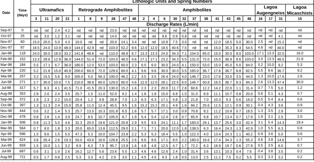
Spring sites are shown in Figure 2, a typical hydrograph in Figure 3, the measured discharge rates in Table 6. In April 1998, August–September 1998 and January 1999, springs were sampled and analyzed. Because we are dealing with mole balances and thus our purpose is to quantify an average of weathering reactions taking place throughout a year, the water
composition of each spring is represented by the mean concentrations of the samples collected in the three periods (Table 7).
In each campaign, three samples were taken from each spring. One 1 L sample was put directly into a polyethylene flask and stored unacidified. Two 125 mL samples were first filtered over a 0.45 m cellulose nitrate filter and then one was acidified with 1 mL of 12 M HCl while the other was stored unacidified. At the sampling site, pH and conductance (Ec) were measured using a PHOX (model 902) portable meter. In a field laboratory, alkalinity was determined by titrating 100 mL of the 1 L sample within one day after collection, using the Gran-plot method for end-point determination. The 125 mL unacidified sample was used
to determine chloride, sulphate and nitrate by ion-chromatography. The acidified sample was used to determine sodium, potassium, magnesium, calcium, sulphur and silica by inductively coupled plasma spectrometry (ICP-AES); sulphur concentrations were multiplied by a factor 3 to obtain the sulphate concentrations. House standards were used for calibration. In all cases, the deviations from charge balance are < 5 %, which is remarkable for dilute waters.
DATA ANALYSIS
Determination of Effluxes of Dissolved Components from Spring Water Data
The flux of a dissolved component (kg/(ha.y)) is the product of a concentration (kg/L) by a annual discharge (L/y) divided a recharge area (ha). In case our hydrogeological system is a small watershed all previous parameters are measurable, but if its a spring in crystalline bedrock the recharge area is difficult to define. Alternatively, we estimated the number of hectares required to rise the average
discharge rate to a certain level (equivalent recharge
area)
by combining one
method of recharge estimation (Appendix 2) with another linking annual recharge, average discharge and recharge area (Figure 4).The Use of Mole balances for the Assessment of Mineral Weathering Rates (the SiB Model)
Mole balances estimated mineral weathering rates in many studies (Velbel, 1985a, 1992; Taylor and Velbel, 1991; Pacheco and Van der Weijden, 1996; Parkhurst, 1997; Pacheco et al., 1999; among others). The most common approaches were reviewed by Pacheco and Van der Weijden (1998), and in this study we used the so-called SiB algorithm introduced by Pacheco and Van der Weijden (1996); the mechanics is outlined in Appendix 3 and the modus operandi described briefly in relation to our study area.
Step 1: Establishment of the Conceptual Geochemical Model - Table 3 (rock mineralogy) and columns 6-7 of Table 4 (soil clays) suggest that hydrolysis of feldspars, amphiboles, chlorites and clinozoisite into mixtures of smectite plus halloysite, dissolution of sphene, olivine, serpentine and talc with subsequent precipitation of titanium and iron oxides and congruent dissolution of calcite are major natural sources of solutes to springs. From land uses (Figure 2, Table 5) we expect that application of manures and fertilizers is an important anthropogenic source of solutes and promote exchange reactions among cations. There is no information on the rates at which the biomass is currently assimilating dissolved components. As a working hypothesis, we assume a steady state between groundwater and the organic compartment.
Step 2 - Match of Spring Compositions with Sets of Weathering Reactions - The SiB
algorithm programs the mixing of two clays from reaction of a single aluminum silicate, but the ability is restricted to a couple of primary phases; the other phases must weather to end-member products or dissolve congruently. Mixtures of clays are represented by the symbolic reaction M cP1+(1-c)P2, where M is the primary mineral, P1 and P2 the clays and 0<c<1.
To generate different sets of weathering reactions, the SiB algorithm increments the c coefficient, and to match them with spring compositions Equation 9 is applied. Whenever a positive solution is attained (j's and u
i
F
's > 0), the set is said a valid SiB solution.Step 3: Check of Results against Boundary Conditions - Usually, a number of valid solutions apply for each spring. The most likely one is the best fit to the following bounds: the "single-spring" condition (or clay test) is applied to each spring separately and states that the
abundances of clays calculated by Equation 10 must approach those in soils nearby the spring. When such detailed information is not available, the next best test is to use the regional distribution of clay minerals (Table 4). In case the single-spring condition fails to give each spring its best-fit solution, the user must consider the "multiple-spring" condition, which sets best-fit solutions by testing all springs simultaneously. The method stands on knowledge
about the composition of locally applied fertilizers and works as follows: (a) Fluxes derived from fertilizers (mostly
F
Cl*,F
SO* 4,F
NO* 3 andF
Cau ) are expected to be high when springs are located in areas with intensive agriculture and low when they are remote from these areas. Besides, because theF
Cl*,* 4
SO
F
andF
NO* 3 are known quantities while the u CaF
is a by-product of the SiB algorithm, it would be possible to use the known fluxes (or their sum in equivalents Pollution) to investigate the congruity of unknownconcentration; (b) This is done by regression analysis. First, allF
Cau 's of a given spring (one for each valid solution) are plotted against the Pollution score of that spring and this step is repeated for all the other springs. Second, a straight line is fitted to the resulting scatter plot and a theoretical best-fitu Ca
F
is calculated for each spring. Third, by comparing the actualF
Cau 's of the springs with their best-fit values, it is possible to select pairs of minimum difference. The valid SiB solutions linked to these actualF
Cau 's are the best-fit solutions.As additional constraints to the SiB solutions, it would be beneficial to have more elements in the set of mole balance equations that could help identify sources of water and solutes, for example Br and(or) Sr and its isotopes. They were not considered because such analyses were not available.
RESULTS AND DISCUSSION
Annual Recharges, Recharge Areas and Effluxes
Applying the methods of Appendix 2 to data in Tables 6 and 7, we determined for all 25 springs the median discharge rate (Qmed), the recharge occurring between 1998 and 1999 (Vr), the recharge area (A), the water discharged during 365 days (V-365; from March 1998 till
February 1999), and the fluxes of dissolved components (
F
it). Results are in Table 8, a stepwise determination is given below for spring nr. 2.Figure 3 is the hydrograph of spring nr. 2. From the baseflow discharge rates (dashed lines), t1 values were obtained for the 1998 and 1999 recessions (320 and 2280 days). Replacement of t1 and associated Q0 values (12.0 and 6.3 L/min; from December 1997 and September 1998) in Equation 5, raised potential groundwater discharges to Vp1 = 2404 m3 and Vp2 = 8993 m3. The baseflow discharge of 1998 was determined from Equation 4 (V = 2050 m3), assuming a recession of t = 266 days (December 1997–August 1998). The water remaining in storage at the end of that period as well as the recharge taking place between recessions were computed from Equations 6 and 7, giving Vs = 355 m3 and VR = 8639 m3. Using Figure 4 in combination with Equation 8 and taking into account the VR and Qmed (0.10 L/s, data in Table 6) values, we estimated the annual recharge in length units (Vr = 12 mm) and the recharge area of the spring (A = 72 ha). Finally, fluxes of dissolved components were calculated from their
concentrations (Table 7), the recharge area (A) and V-365 (3351 m3, Table 6).
Match of Water Chemistries with Sets of Weathering Reactions
No information was available about the average composition of local wet and dry depositions. For that reason, the *-fluxes in Equation 9 were replaced by t-fluxes, meaning that the
atmospheric inputs are lumped together with pollution. The SiB algorithm was applied to all 25 springs. We could not link sets of weathering reactions to samples nrs. 6, 32 and 38 and sample nr. 28 gave anomalous results. For the amphibolites and ultramafics, sets were established for the essential rock-forming minerals (Table 3, except quartz) while in the Lagoa units spring compositions matched reactions of plagioclase and chlorite. Mixtures of smectite plus halloysite were considered for plagioclase and chlorite (Lagoa units),
amphibolites and retrograde amphibolites, additional incongruent reactions were set for chlorite and clinozoisite. In both cases they were written to smectite because reactions to halloysite violated the clay test. The compositions of local smectites were not known. Among the typical dioctahedral series (beidellite, montmorillonite and nontronite; compositions in Loughnan, 1969), we adopted beidellite (Ca0.35Al4(Si7.3Al0.7)O20(OH)4) to be secondary
product of plagioclase, hornblende, clinozoisite and ripidolite-RA, and nontronite (Ca0.35Fe4(Si7.3Al0.7)O20(OH)4) to be secondary product of ripidolite-M, picnochlorite,
tremolite and peninnite, because these choices gave us the best match between predicted and real abundances of weathering products.
Check of Results against Boundary Conditions
Table 9 lists the end-member reactions used in the SiB modelling (R1R26), Table 10 depicts
the SiB results. Because multiple sets of weathering reactions agreed with the chemical compositions of springs, we selected best-fit sets by testing them against the predefined boundary conditions: (Clay test) Columns 3–5 of Table 10 contain the best-fit clay mineral abundances. Reactions of ripidolite-M and picnochlorite had to form a small amount of nontronite (< 15%) so they could match the water compositions, notwithstanding the fact that 14 Å clays did not show up in X-ray diffraction analyses on C-horizons of the Lagoa units. For the other lithologic units, predicted and real clay mineral abundances match closely; (Multiple-spring condition) The clay test detected a single best-fit SiB solution for each spring. Still, we determined the regression between Pollution and the best-fit
F
Cau fluxes:F
CauBest-Fit SiB Solutions
The best-fit weathering reactions are shown in column 6 of Table 10. The Ris are in
agreement with column 1 of Table 9 and reactions can be interpreted as illustrated for spring nr. 2 (first in the amphibolites). In this case, the natural water chemistry may be explained by simultaneous weathering of andesine-An45 into 80% beidellite plus 20% halloysite
(0.8R5+0.2R6), of hornblende into 20% beidellite plus 80% halloysite (0.2R7+0.8R8), of
chlorite and clinozoisite into beidellite (R13 and R20) and of sphene into titanium oxides (R22),
accompanied by congruent dissolution of calcite (R23). Columns 7–15 contain the calculated
weathering rates; similar minerals (e.g. ripidolites, picnochlorite and peninnite) were gathered into groups (chlorite) to facilitate further discussion.
Correlation Between Weathering Rates and Recharge Rates
Monitored springs link to very different drainage conditions set by the range of calculated recharge rates (3.5 < Vr < 400 mm/y; Table 8). Huge variations in the annual recharge are justified because we are dealing with very small drainage basins shaped on fractured rocks: most probably, the highest and lowest Vr scores link to densely and sparsely fractured basins,
i.e. to highly and poorly permeable environments. Weathering rates (Table 10) of all minerals correlate with the annual recharge rates; Figure 5 illustrates that for plagioclase and
amphibole. This observation is consistent with the Loughnan’s (1969) statement: "the most important single factor controlling the rate of breakdown of parent minerals and the genesis of specific secondary products is the quantity of water leaching through the weathering
environment", and suggests that weathering rates in the Morais massif are not controlled directly by mineral dissolution rates far from equilibrium, but by either a chemical affinity effect or a transport process (Drever and Clow, 1995; White, 1995).
Normalized Mineral Weathering Rates
Scatter in Figure 5 suggests that factors other than recharge (e.g. bulk percentage and(or) grain size of the minerals) may play an important role in determining the observed weathering rates. Using the information in Table 3 we normalized the rates by mineral abundances. Results are summarized in Figure 6. Normalized rates obtained for plagioclase (0.9–45 moles/(ha·y%plagioclase)) compare favorably with the results of Cleaves et al. (1970), Paces (1983) and Velbel (1985a), which are 14.0, 11.7 and 36.7–39.3 moles/(ha·y·%plagioclase), respectively. Results pertaining to the other minerals were not compared because in most weathering studies the information about spring discharges and(or) mineral abundances is lacking. Minerals were put in ascending order of their maximum weathering rates from the bottom to the top of Figure 6. At the rightmost part we plotted ranks of the Persistence Order of Minerals (POM; Pettijohn, 1941). According to this index, the most stable mineral is anatase (POM = -3) and the least stable is olivine (POM = 22). Despite the fact that only a few of our minerals were included in the POM scale, there is no doubt about the agreement between the normalized rates and the POM ranking.
Immobilization plus Uptake
The conceptual geochemical model assumes a steady state between groundwater and biomass. Violation of this assumption upsets especially the
F
SOt 4,t NO
F
3 and,
u
F
fluxes as we shall discuss in the next paragraphs.From inspection of Tables 1 and 3, it is unlikely that chloride and sulphate in spring waters result from rock weathering. Thus, the Ft fluxes of chloride, sulphate and nitrate as well as the Fu fluxes of magnesium and calcium must match the atmospheric plus fertilizer inputs. The Fad fluxes were estimated from rainwater analyses of a nearby region (Sousa Oliveira, 2001).
They are:
F
Clad = 0.87,F
SOad4 = 1.08,F
NOad3 = 0.14,F
Mgad = 0.14 andF
Caad = 0.94 kg/(ha.y). The inputs from fertilization were determined by: F* = Ft - Fad and Fu* = Fu - Fad.The
F
Cl* andF
SO*4 fluxes are related to application of Foskamónio in potato and maize fields (Table 5). If the steady state hypothesis is acceptable, a scatter plot of these fluxes defines a straight line of slope 3.831 intercepting the origin (3.831 is the sulphate to chloride wt. ratio in Foskamónio). In Figure 7, bullets are theF
Cl* andF
SO* 4 fluxes of spring waters and the dotted line's slope is 3.831. In most cases bullets fall below the dotted line, i.e. the hypothesis is unsustainable. Besides, because chloride is a conservative ion, deviations from the dotted line link to diminishments in the sulphate fluxes promoted by immobilization (incorporation into microorganisms), uptake (assimilation by natural vegetation and crops) or volatilization. In the thin, relatively well drained and aerated soils of Morais, the anaerobic conditions necessary for sulphate reduction will not prevail, thus sulphur volatilization is supposedly negligible. Sulphate decrease in groundwater must therefore reflect the retention by the organic compartment. The relation between theF
SO* 4 fluxes and those due to immobilization plus uptake (F
SOo 4) or to application of Foskamónio (F
SOp4) is understood from Figure 7.A similar plot is not applicable to nitrate, magnesium or calcium because sources other than Foskamónio (manure and Nitrolusal, Table 5) contribute to their F*(Fu*) fluxes and the Fu* fluxes may be influenced by cation exchange reactions. Alternatively, we used the element matching technique (Melillo and Gosz, 1983) that is based on the mean N/S, N/Mg and N/Ca ratios in soil, vegetation and crops (averages: 9.54, 10.34 and 4.81, as compiled from
Whitehead, 1964; Rodin and Bazilevish, 1967; Cole and Rapp, 1981; Melillo and Gosh, 1983; Wild, 1988; Brady, 1990; Schlesinger, 1991). In agreement with it and by assuming that nitrogen and sulphur are provided to organisms and plants by nitrate and sulphate in the soil solution, the uptake of 1 kg/(ha.y) of sulphate must be accompanied by the uptake of 14.08
kg/(ha.y) of nitrate (
9
.
54
32
/
96
14
/
62
, where 62, 14, 96 and 32 are the masses of nitrate,
nitrogen, sulphate and sulphur in g/mol). In general, the Cao o
Mg o
NO F F
F 3, and fluxes may be
computed sequentially by: NOo
o Ca o NO o Mg o SO o NO F F F F F F 314.08 4, 0.022 3and 0.047 3.
Applying the element matching technique to our data, we found the highest
F
NOo 3 flux (theone representing abundant manuring and fertilization) to approach 834 kg/(ha.y) of NO3 (188
kg/(ha.y) of N), a value that is consistent with the range measured by Bashkin et al. (1986) for plant uptake in a small agricultural catchment (131.9–183.2 kg/(ha.y) of N).
Cation Exchange
Using a [Mg]p/[Ca]p versus [SO4]t/[NO3]t plot, Pacheco et al. (1999) illustrated how cation
exchange reactions modified the chemistry of shallow groundwaters from granites in northern Portugal. Replacing concentrations by fluxes we drew Figure 8; circles mark the fluxes, stars the equivalent Mg/Ca and SO4/NO3 ratios in manure (0.82 and 0.18, Table 5), Foskamónio
(0.02 and 3.84) and Nitrolusal (0.01 and 0.00); the mixing and dotted lines describe the Fp fluxes in case they result solely from the application of manure and Foskamónio or from an equilibrium with the soil exchange complex.
Spring waters are not in equilibrium with the soil exchange complex because circles deviate from the dotted line. One sample may relate to simultaneous application of manure,
Foskamónio and Nitrolusal as the circle falls in the "triangle" defined by the stars. The other circles are above the mixing line which is interpreted as follows: exchange reactions are actively displacing Mg from the exchange sites (raising the *
/
Cap*p Mg
F
F
ratios) as aconsequence of application of calcium rich fertilizers. The highest deviations from the mixing line occur when the sulphate to nitrate ratios are close to those found in manure, decreasing rapidly as the ratios increase towards the ones found in Foskamónio. This trend is represented
schematically by the dashed line and may be interpreted as follows: (1) When only in situ generated organic (humus) plus inorganic (clay minerals) constituents play a role in the exchange of Mg by Ca, the impact of this reaction on the FMgp*/FCap* ratios is low, expressed in the segment of the dashed line that is parallel to the mixing line; (2) This impact becomes higher when additional amounts of organic compounds are incorporated into the soil system by manuring. The more abundant manuring is, the higher this impact will become, resulting in the quasi vertical segment of that line.
Nutrient Balances and Changes in Soil Water Alkalinity
It should be noted that changes in alkalinity promoted by botanical uptake were not accounted for in the mole balance of bicarbonate (Equation 9). When cations such as Mg2+ and Ca2+ are removed from the soil solution in excess of the uptake of negatively charged ions, the plants release H+ to maintain internal balance of charge. This H+ may in turn reduce the alkalinity and(or) replace cations in the exchange sites driving them into the soil solution. On the other hand, when plants consume anions such as SO4
and NO3
-in excess of positively charged ions they release HCO3
to keep charge balance. In both cases, the uptake process has
consequences on soil water composition: uptake of cations may reduce while uptake of anions increases alkalinity, the overall change being dependent on how much nutrients of either type are incorporated into plant tissue. We believe that in a region dominated by rocks of low resistance to weathering (serpentinites, amphibolites) biological processes have relatively little effect on the general level of alkalinity acquired by water-mineral interactions under soil PCO2. Processes such as ammonium oxidation (nitrification) may also reduce spring water alkalinity. A redox equation on ammonium-nitrate was not included in the mole balance model because, except sporadically, external sources of NH4
+
CONCLUSIONS
Assuming that silicic acid (Si) and bicarbonate (B) in spring waters are the result of chemical weathering, we applied our SiB algorithm to reconstruct the weathering reactions of minerals (of known composition), present in five lithologic units of the Morais massif that contributed to the water composition. Hydrolysis of feldspars, amphiboles, chlorites and clinozoisite yielded mixtures of smectites and halloysite, hydrolysis of olivine, serpentine, talc and sphene produced titanium and iron oxides, whereas calcite dissolved congruently. Beidellite and nontronitetheir compositions adopted from literaturewere used as representatives of the smectites giving the best SiB results. The best-fit weathering reactions are combinations of reactions water and carbon dioxide with individual minerals and selected on the basis of meeting the boundary conditions posed by the mineralogy of soils developed on the parent rocks and by contributions of fertilizers used in the area.
Linkage of annual recharge, average spring discharge and recharge area allowed to calculate the discharge in volume per recharge area within a lithologic unit per year. Combination of the derived weathering reactions, the normalized discharge and knowledge of the
mineralogical composition of the rocks, made possible the calculation of the weathering rates of the rock-forming minerals as moles/(ha.y.%mineral). We obtained the following order of these normalized weathering rates in the Morais massif: forsterite (485) > calcite (266) > clinozoisite (114) > talc (108) > sphene (98) > chlorite (49) > plagioclase (45) > amphibole (28) > serpentine (19).
Overall, the contribution of natural chemical weathering, represented by the bicarbonate concentration, by far exceeds contributions of other sources, represented by chloride, sulphate and nitrate concentrations. Other sources being considered are atmospheric deposition, application of manure and industrial fertilizers. It had to be taken into account that selective
in the soil compartment can change the original chemical signature of these sources. Using data on the composition of atmospheric deposition and on the most frequently applied
fertilizers, literature data on the ratios of storage of nitrogen, sulphur, calcium and magnesium in vegetation, and ratios of the latter components in solution, it was possible to reconstruct the (modified) contributions of these other sources to the spring-water compositions.
ACKNOWLEDGEMENTS
We thank the associate editor R.L Bassett and the reviewer Art F. White for their comments and suggestions. They were of great help in the improvement of an earlier version of this paper. We also thank Luís Gens for the help with the drawings.
APPENDIX 1 – THE BALANCE OF CATION PROPORTIONS
The method we call the Balance of Cation Proportions computes the weight percentages of minerals in a rock sample. It stands on the solution of a set of linear equations, which in matrix form is written as:
B
AX
(1)where A is a matrix of structural compositions, B an array of cation proportions and X an array of mineral weight percentages.
Equation 1 is solved by Singular Value Decomposition (SVD) as described in Press et al. (1989). First, a matrix A is built. This is a square matrix where the number of non-zeroed rows (n) equals the number of elements describing the chemistry of rock-forming minerals (e.g. Si, Ti), and the number of non-zeroed columns (m) equals the number of minerals in each rock sample (e.g. plagioclase, amphibole). For n > m, the set of linear equations is overdetermined and SVD provides a solution using a least-squares method. For n = m, the set has likely a unique solution. Finally, for n < m, the set is undetermined and SVD provides a solution which minimizes the modulus of X (X). The aij's (elements of A) quantify the number of moles of element i in one mole of mineral j and can be read directly from the structural formulas of the minerals. After matrix A is built, a B array is composed for each rock sample. The bj's are the cation proportions of each chemical component and are determined by dividing the weight percentage of each oxide by its equivalent molecular weight. Once a positive solution of Equation 1 is obtained, using A and B as defined above, the mineral weight percentages are computed from the X array by multiplying each xj by the molecular weight of the corresponding mineral and converting the results into percentages.
APPENDIX 2 – DETERMINATION OF RECHARGE AREAS FROM SPRING WATER DATA
The approach we used to estimate the recharge area of a spring combines a method for recharge estimation (Domenico and Schwartz, 1990) with a method linking annual recharge, average spring discharge and recharge area (Figure 4).The first method assumes that during a recession period baseflow discharge rates obey an exponential law of the type:
kt
e
Q
Q
0 (2)where Q is the baseflow discharge rate at instant t, Q0 the same rate but at the beginning of the recession and k the recession constant. Accordingly, a plot of baseflow discharge rates against time on a semilogarithmic paper (log Q vs. t) yield a straight line, the slope of which defines the recession constant. For this case, the recession expression may be rewritten as:
1 / 0
10
t tQ
Q
(3)where t1 is the time corresponding to one log cycle of Q. The volume (V) of baseflow discharge corresponding to a given recession is found by integrating Equation 3 over the times of interest:
tQ
t tdt
Q
t
t tV
0 / 1 0 / 0 1 110
1
1
3
.
2
10
(4)The recharge (m3) occurring between two recession periods is estimated by a stepwise procedure which incorporates the next four consecutive steps: (1) Calculate the potential groundwater discharge at the beginning of the first recession, i.e. the volume of groundwater that would be discharged by baseflow if complete depletion took place without interruption, or—in other words—the water in storage at the beginning of the first recession. This is done by considering t = in Equation 4:
3
.
2
1 0 1t
Q
V
p
(5)where Vp1 is the potential groundwater discharge; (2) Calculate the water in storage at the end of the first recession (Vs). This is simply the difference between Vp1 and V:
V
V
V
s
p1
(6)(3) Calculate the potential groundwater discharge at the beginning of the second recession (Vp2). This is done by applying Equation 5 to the new Q0 and t1; (4) Finally, calculate the recharge that took place between recessions (VR); this is the difference between Vp2 and Vs:
s p
R
V
V
V
2
(7)The second method establishes a relation between the medium discharge rate (L/s), the annual recharge (mm) and the recharge area (ha) of a particular spring. It is readily understood that recharge areas cannot be determined directly from known median discharge rates plus calculated VR's, because annual recharges in Figure 4 are expressed in mm while VR's are expressed in m3. But they can be determined by the following iterative procedure: (1) Assume a value for the annual recharge in mm (Vr); (2) Determine analytically the recharge area (A) by the formula:
r R c
V
V
A
(8)where subscript c means calculated; (3) Use the median discharge rate (Qmed) in combination with the assumed Vr to determine graphically (from Figure 4) the recharge area (Ag, where subscript g means retrieved from the plot); (4) Compare Ac with Ag. If they are equal, the procedure stops, because we have found the best A (Ac or Ag) and Vr values. Otherwise, start again from step 1, assuming a new Vr, until Ac = Ag.
APPENDIX 3 – AN OUTLINE ON THE MECHANICS OF THE SIB ALGORITHM
When working with fluxes, the SiB algorithm uses the following mole and charge balance equations:
cations k u k m j u i j ij ad i t i i k NO S O Cl F F z F F Pollution n i F r F F F 1 * * * 1 * 3 4 2 ) ,..., 1 (
(9)where: n is the number of dissolved components assumed to have affinities with chemical weathering (n = 6, Na+, K+, Mg2+, Ca2+, HCO3- and H2SiO3), cations is the number of major cations in the chemical system (cations = 4, Na+, K+, Mg2+, Ca2+) and m is the number of reactant phases;
F
it is the total and*
i
F
is a net flux of dissolved component i, which include the fluxes derived from atmospheric deposition (F
iad) and unspecified sources (F
iu), all expressed in mol/(hay); rij is the ratio between the stoichiometric coefficients of dissolved component i and reactant phase j and j is the weathering rate of reactant phase j (mol/(hay)); zk is the charge of cation k.The set has 7 (n+1) equations. The unknowns are the m reactant phases plus the Fu fluxes. Because the algorithm considers Fu fluxes only for the four major cations, the number of unknowns is written as
m+4. Accordingly, if m = 3, Equation 9 is determined and SVD (Appendix 1) provides unique values
for the unknowns, but if m < 3 or m > 3, the set is over or undetermined and SVD can only find least squares or minimum estimates for them.
Once weathering rates are calculated, the SiB algorithm uses them in combination with rlj ratios, now between the stoichiometric coefficients of secondary product l and primary mineral j, to predict the amounts of clay minerals being produced by weathering:
j ij ij
r
(10)with l = 1,...,p, where p is the number of weathering products derived from primary mineral j (1 or 2 are allowed) and lj is the rate at which secondary product l is being formed as a consequence of the rate at which primary mineral j is being weathered.
REFERENCES
Agroconsultores and Coba, 1991. Carta de solos, carta do uso actual da terra e carta de aptidão da terra do nordeste de Portugal. Technical Report, Trás-os-Montes and Alto Douro University, Vila Real, 311p.
Appelo, C.A.J., Postma, D., 1993. Groundwater, geochemistry and pollution. Balkema, Rotterdam. Bashkin, V.N., Mocik, A., Skorepova, I., Kudeyarov, V.N., Nikitishen, V.I., 1986. Application of nitrogen fertilizers and state of the environment. In: Nitrogen balance and transformation of nitrogen fertilizers in soils. Puschino, pp. 104-154.
Brady, N.C., 1990. The nature and properties of soils (10th edition). Macmillan Publishing Company, New York, and Collier Macmillan Publishers, London.
Cleaves, E.T., Godfrey, A.E., Bricker, O.P., 1970. Geochemical mass balance of a small watershed and its geomorphic implications. Geol. Soc. Am. Bull. 81, 3015–3032.
Cole, D.W., Rapp, M., 1981. Elemental cycling in forest ecosystems. In: Reichle, D.E. (Ed.), Dynamic properties of forest ecosystems, Cambridge University Press, Cambridge, pp. 341-409 (Chapter 6). Domenico, P.A., Schwartz, F.W., 1990. Physical and chemical hydrogeology. John Wiley & Sons Inc., New York.
Drever, J.I., Clow, D.W., 1995. Weathering rates in catchments. In: White, A.F., Brantley, S.L., Chemical weathering rates of silicate minerals. Reviews in mineralogy, vol. 31, Mineralogical Society of America, Washington DC, pp. 463–483 (Chapter 10).
Garrels, R.M., Mackenzie, F.T., 1967. Origin of the chemical compositions of some springs and lakes. In: Stumm, W. (Ed.), Equilibrium concepts in natural water systems. Am. Chem. Soc., pp. 222– 242.
Hornung, M., Rodá, F., Langan, S.J. (Eds.), 1990. A review of small catchment studies in Western Europe producing hydrogeochemical budgets. Air Pollution Report 28, Commission of the European Communities, 186 pp.
Hutchison, C.S., 1974. Laboratory handbook of petrographic techniques. John Wiley & Sons Inc., New York.
Likens, G.E., Bormann, F.H., 1995. Biogeochemistry of a forested ecosystem (2nd edition). Springer Verlag Inc., New York.
Likens, G.E., Driscoll, C.T., Buso, D.C., Siccama, T.G., Johnson, C.E., Lovett, G.M., Fahey, T.J., Reiners, W.A., Ryan, D.F., Martin, C.W., Bailey, S.W., 1998. The biogeochemistry of calcium at Hubbard Brook. Biogeochemistry 41, 89–173.
Loughnan, F.C., 1969. Chemical weathering of the silicate minerals. American Elsevier Publishing Company Inc., New York.
Marques, F.G., Ribeiro, A., Pereira, E., 1992. Tectonic evolution of the deep crust: Variscan reactivation by extension and thrusting of Precambrian basement in the Bragança and Morais massifs (Trás-os-Montes, NE Portugal). Geodynamica Acta 5, 135–151.
Melillo, J.M., Gosz, J.R., 1983. Interactions of biogeochemical cycles in forest ecosystems. In: Bolin, B., Cook, R.B. (Eds.), The major biogeochemical cycles and their interactions. SCOPE, Wiley, New
Moldan, B., Cerný, J., 1994. Small catchment Research. In: Moldan, B., Cerný, J. (Eds.),
Biogeochemistry of small catchments: a tool for environmental research. SCOPE 51, John Wiley & Sons Inc., Chichester, pp. 1–29 (Chapter 1).
Nelson, D.W., Sommers, L.E., 1982. Total carbon, organic carbon and organic matter. In: Page, A.L. (Ed.), Methods of soil analysis. ASA, SSSA, Madison, Wisconsin, pp. 539–580 (Chapter 29).
Paces, T., 1983. Rate constants of dissolution derived from the measurements of mass balance in hydrological catchments. Geochim. Cosmochim. Acta 47, 1855–1863.
Paces, T., 1986. Rates of weathering and erosion derived from mass balance in small drainage basins. In: Colman, S.M., Dethier, D.P. (Eds.), Rates of chemical weathering of rocks and minerals, Academic Press Inc., Orlando, pp. 531–550 (Chapter 22).
Pacheco, F.A.L., 2000. Hidrogeologia em maciços de rochas cristalinas (Morais - Chacim - Macedo de Cavaleiros): bases para a gestão integrada dos recursos hídricos da região. Ph.D Thesis, Universidade de Trás-os-Montes e Alto Douro, Vila Real, 395 pp.
Pacheco, F.A.L., Van der Weijden, C.H., 1996. Contributions of water–rock interactions to the composition of groundwater in areas with a sizable anthropogenic input. A case study of the waters of the Fundão area, central Portugal. Water Resour. Res. 32, 3553–3570.
Pacheco, F.A.L., Van der Weijden, C.H., 1998. Past, present and future of geochemical input–output budgets. In: The Eighth Annual VM Goldschmidt Conference, Paul Sabatier University, Toulouse, France. Mineralogical Magazine (abstracts volume), vol. 62A, part 2, pp. 1120–1121.
Pacheco, F.A.L., Sousa Oliveira, A., Van der Weijden, A.J., Van der Weijden, C.H., 1999. Weathering, biomass production and groundwater chemistry in an area of dominant anthropogenic influence, the Chaves–Vila Pouca de Aguiar region, North of Portugal. Water, Air Soil Pollut. 115, 481–512.
Parkhurst, D.L., 1997. Geochemical mole–balance modeling with uncertain data. Water Resour. Res. 33, 1957–1970.
Pereira, E., Ribeiro, A., Silva, N., 1998. Carta Geológica de Portugal, folha 7D (Macedo de Cavaleiros). Publicações do Instituto Geológico Mineiro-Ministério da Economia.
Pettijohn, F.G., 1941. Persistence of heavy minerals and geologic age. J. Geol. 49, 610–625.
Portugal Ferreira, M.R., Forster, I.H., 1989. Geological field trip in Portugal. Unpublished excursion guide, Coimbra University, 49 pp.
Press, W.H., Flannery, B.P., Teukolsky, S.A., Vetterling, W.T., 1989. Numerical recipes in Pascal, Cambridge University Press, Cambridge.
Rhoades, J.D., 1982. Cation exchange capacity. In: Page, A.L. (Ed.), Methods of soil analysis. ASA, SSSA, Madison, Wisconsin, pp. 149–158 (Chapter 8).
Ribeiro, A., 1974. Contribution à l'étude tectonique de Trás-os-Montes Oriental. Memórias dos Serviços Geológicos de Portugal, vol. 24 (Nova Série), 177 pp.
Ribeiro, A., 1997. Maciço de Morais. Excursion guide, XIV reunião de geologia do Oeste Peninsular, pp. 11–27.
Ribeiro, A., Pereira, E., Dias, R., 1990. Structure in the NW of the Iberian Peninsula. In: Dallmeyer, R.D., Martinez, E. (Eds.), Pre-Mesozoic Geology of Iberia. Springer Verlag, New York, pp. 220–236 (Chapter 3.1).
Rodin, L.E., Bazilevish, N.I., 1967. Production and mineral cycling in terrestrial vegetation. Oliver and Boyd, Edinburg and London.
Schlesinger, W.H., 1991. Biogeochemistry (2nd Ed.). Academic Press, San Diego.
Sousa Oliveira, A., 2001. Hidrogeologia dos sistemas gasocarbónicos da província hidromineral Transmontana: Ribeirinha (Mirandela), Sandim (Vinhais) Segirei e Salgadela (Chaves). Unpublished PhD Thesis, Universidade de Trás-os-Montes e Alto Douro, Vila Real, 442p.
Taylor, A.B., Velbel, M.A., 1991. Geochemical mass balances and weathering rates in forested watersheds of the Southern Blue Ridge: II - Effects of botanical uptake terms. Geoderma 51, 29–50. Thomas, G.W., 1982. Exchangeable cations. In: Page, A.L. (Ed.), Methods of soil analysis. ASA, SSSA, Madison, Wisconsin, pp. 159–166 (Chapter 9).
Todd, D.K., 1980. Groundwater hydrology. John Wiley & Sons Inc., New York.
Velbel, M.A., 1985a. Geochemical mass balances and weathering rates in forested watersheds of the Southern Blue Ridge. Am. J. Sci. 285, 904–930.
Velbel, M.A., 1985b. Hydrochemical constraints on mass balances in forested watersheds of the Southern Appalachians. In: Drever, J.I. (Ed.), The chemistry of weathering. Proc. NATO Adv. Res. Workshop, July 1984, Reidel Publ., Dordrecht, Netherlands, pp. 231–247.
Velbel, M.A., 1986. The mathematical basis for determining rates of geochemical and geomorphic processes in small forested watersheds by mass balance: examples and implications. In: Colman, S.M., Dethier, D.P. (Eds.), Rates of chemical weathering of rocks and minerals. Academic Press Inc., Orlando, pp. 439–451 (Chapter 18).
Velbel, M.A., 1992. Geochemical mass balances and weathering rates in forested watersheds of the Southern Blue Ridge: III - Cation budgets and the weathering of amphibole. Am. J. Sci. 292, 58–78. Velbel, M.A., 1993. Constancy of silicate-mineral weathering-rate ratios between natural and experimental weathering: implications for hydrologic control of differences in absolute rates. Chem.Geol. 105, 89–99.
Velbel, M.A., 1995. Interaction of ecosystem processes and weathering processes. In: Trudqill, S.T. (Ed.), Solute modelling in catchment systems, John Wiley & Sons Inc., Chichester, pp. 193–209. White, A.F., 1995. Chemical weathering rates of silicate minerals in soils. In: White, A.F., Brantley, S.L. (Eds.). Chemical weathering rates of silicate minerals. Reviews in mineralogy, vol. 31,
Mineralogical Society of America, Washington DC, pp. 407-461 (Chapter 9).
Whitehead, D.C., 1964. Soil and plant-nutrition aspects of the sulphur cycle. Soils and Fertilizers 27, 1-8.
Table 1
Caption: Average chemical compositions and corresponding molecular weights of
minerals in lithologic units of the Morais massif. Other minerals in the Lagoa units
and amphibolites sensu lato. include quartz and calcite. Their theoretical structural
formulas and corresponding molecular weights are: SiO
2(60.1) and CaCO
3(100.1).
Mineral n Average Structural Formula Molecular Weight
Albite 11 NaAlSi3O8 262.2
Muscovite 3 (Na0.3K1.7)(Al3.6Fe0.2Mg0.2)(Si6.3Al1.7)O20(OH)4 797.4
Chlorite (Ripidolite)-M 6 (Al2.8Fe5.6Mg3.6)(Si5.3Al2.7)O20(OH)16 1289.6
K-Feldspar Phenoblasts 2 KAlSi3O8 278.3
Albite Phenoblasts 4 NaAlSi3O8 262.2
Average Plagioclase 12 Na0.7Ca0.3Al1.30Si2.7O8 265.1
Chlorite (Picnochlorite) 6 (Al2.9Fe6.1Mg3.0)(Si5.8Al2.2)O20(OH)16 1306.2
Muscovite 7 (Na0.1K1.9)(Al3.4Fe0.35Mg0.25)(Si6.5Al1.5)O20(OH)4 805.0
Hornblende-A 23 Na0.4Ca2(Al0.7Fe1.6Mg2.7)(Si6.7Al1.3)O22(OH)2 872.5
Average Plagioclase 30 Na0.55Ca0.45Al1.45Si2.55O8 269.4
Clinozoisite-A 2 Ca2Al2.6Fe0.4Si3O12(OH) 465.9
Hornblende-RA 20 Na0.5Ca2(Al0.7Fe1.5Mg2.8)(Si6.9Al1.1)O22(OH)2 871.8
Albite 13 NaAlSi3O8 262.2
Clinozoisite-RA 13 Ca2Al2.5Fe0.5Si3O12(OH) 468.8
Chlorite (Ripidolite)-RA 16 (Al2.6Fe3.6Mg5.8)(Si5.5Al2.5)O20(OH)16 1226.2
Sphene 10 CaTiSiO5 196.1
Forsterite 14 (Mg1.78Fe0.22)SiO4 147.6
Serpentine 13 (Mg2.75Fe0.25)Si2O5(OH)4 285.0
Talc 8 (Mg5.9Fe0.1)Si8O20(OH)4 761.7
Tremolite 10 Ca2(Mg4.8Fe0.2)(Si7.95Al0.05)O22(OH)2 818.6
Chlorite (Penninite) 18 (Al1.8Fe0.6Mg9.6)(Si6.4Al1.6)O20(OH)16 1130.4
n - Number of electron microprobe analyses
Ultramafics (Serpentinites with Tremolite+Chlorite Bands) Retrograde Amphibolites
Lagoa Micaschists
Lagoa Augengneisses
Table 2
Caption: Average chemical compositions of lithologic units in the Morais massif;
values in wt.%.
SiO2 TiO2 Al2O3 Fe2O3 MnO MgO CaO Na2O K2O P2O5 LOI Total
60.1 79.9 51.0 79.9 70.9 40.3 56.1 31.0 47.1 71.0 Lagoa Micaschists 6 68.4 0.7 14.5 5.0 0.0 1.3 0.5 2.3 2.4 0.1 3.8 98.9 Lagoa Augengneisses 6 70.2 0.5 14.0 3.1 0.0 0.6 1.8 3.1 3.3 0.2 2.2 99.0 Amphibolites 8 48.5 1.1 15.6 9.5 0.2 8.3 10.9 2.3 0.1 0.1 2.8 99.3 Retrograde Amphibolites 10 47.8 1.6 15.4 11.0 0.2 6.6 10.6 2.7 0.1 0.1 3.1 99.1 Tremolite+Chlorite Bands 3 47.1 0.5 4.1 7.9 0.2 24.8 7.8 0.1 0.0 0.2 5.7 98.4 Serpentinites 5 39.4 0.1 2.0 8.5 0.1 34.2 0.4 0.0 0.0 0.0 14.0 98.8
n - Number of rock samples
Oxide Percentages in the Lithologic Units Oxide Equivalent Weights Lithologic Unit n
Table 3
Caption: Average mineralogical compositions of lithologic units in the Morais
massif. Values in wt.%, calculated by the Balance of Cations Proportions (Appendix
1).
Quartz Albite Muscovite Chlorite
Lagoa Micaschists 43.4 18.1 25.9 12.6
K-Feldspar Phenoblasts
Albite
Phenoblasts Quartz Plagioclase Chlorite Muscovite Lagoa Augengneisses(a) 17.6 (20.3) 6.5 (6.5) 35 (34.8) 29.2 (30.4) 8.2 (4.5) 3.5 (3.1)
Hornblende Plagioclase Clinozoisite Chlorite Sphene Calcite Quartz
Amphibolites 56.5 24.8 3.3 7.4 2.7 trace(b) 5.3
Retrograde Amphibolites 35.0 17.3 22.5 13.9 3.9 trace(b) 7.4 Forsterite Serpentine Talc Tremolite Chlorite
Serpentinites (S) trace(b)
67.4 32.6
Tremolite + Chlorite Bands (B) 75.0 25.0
Mixture 0.63 S + 0.37 B(c) trace(b) 42.5 20.5 27.7 9.3
(a)
Values within brackets obtained with the CIPW norm; 6.5% of the calculated albite was linked to the phenoblasts, the remaining was added to anorthite to obtain matrix plagioclase (giving An26); Picnochlorite = Hematite + Rutile + Hypersthene; Muscovite = Corundum. (b)
< 1%; assumed equal to 1% in the calculation of normalized weathering rates (Figure 6).
(c)
Based on the number of samples representing serpentinites and tremolite+chlorite bands (Table 2).
Mineralogical Composition Lithologic Unit
Table 4
Caption: Physical and chemical properties of saprolitic materials derived from the
main lithologic units of the Morais massif.
Smectite Halloysite [Ca-S] [Mg-S] [K-S] [Na-S]
Lagoa Micaschists 3 0.6 5.5-6.0 SL 0.0 100.0 3.5 0.8 0.1 0.0 5.1 Lagoa Augengneisses 3 0.9 5.9-7.0 L 0.0 100.0 0.9 0.9 0.2 0.0 2.2 Amphibolites 4 0.4 6.0-7.0 L 85-45 15-55 4.7 1.0 0.1 0.1 6.2 Retrograde Amphibolites 5 0.4 5.0-6.9 SL 80-50 20-50 5.2 0.7 0.1 0.1 6.7 Ultramafics 4 0.7 6.8-7.8 L 65-50 35-50 3.4 0.5 0.2 0.1 4.2
n - Number of saprolite samples. OM - Organic Matter.
L - Loamy; S - Sandy.
Smectite and Halloysite ranges estimated on the basis of X-Ray diffraction 14Å and 7.2Å peak heights. [X] - Concentration of cation X in meq/100g of dried soil; S - soil exchanger.
CEC-pH7 (meq/100g) - Cation Exchange Capacity at soil pH of 7.
Lithologic Unit n OM
(%) pH-H2O Texture
Exchange Bases
CEC-pH7 Clay Types (%)
Table 5
Caption: Average chemical compositions and common applications of locally applied
fertilizers; values in wt. %. Source: Pacheco et al. (1999).
Cow Manure Nitrolusal (a) Foskamonio10-10-10 All Crops Rye, Pastures Potato, Maize
H2O 70.00 0.00 0.00 Organic Matter 26.00 0.00 0.00 Na 0.00 0.04 1.53 K 0.74 0.07 7.56 Mg 0.06 0.01 0.37 Ca 0.12 1.34 30.09 Cl 0.00 0.63 7.91 SO4 0.45 0.00 30.30 NO3 3.14 75.20 10.19 NH4 0.00 22.50 0.00 PO4 0.00 0.00 10.08 Sr 0.00 0.01 1.90 Total 100.51 99.80 99.93 (a) Sporadic application Component
Table 6
Caption: Discharge rates of the monitored springs.
Lagoa Micaschists 3 11 20 21 1 8 9 28 47 48 2 4 6 30 32 37 38 41 43 45 46 16 17 31 15 Sep-97 0 nd nd 2.4 4.2 nd nd nd 23.0 nd nd nd nd nd nd nd nd nd nd nd nd nd nd nd nd nd Oct-97 25 nd 3.0 1.2 3.1 nd nd nd 14.0 nd nd nd nd 9.6 0.9 0.8 nd nd nd nd nd nd nd nd 4.1 nd Nov-97 60 15.0 20.0 5.0 4.3 10.0 nd nd 20.0 14.1 3.4 nd nd 10.9 7.5 3.0 nd nd 12.0 18.5 5.0 30.0 2.5 nd 15.2 nd Dec-97 87 18.5 24.0 10.9 48.0 144.0 42.9 nd 103.0 52.2 8.6 12.0 12.0 18.5 40.6 7.5 nd nd 15.0 35.3 8.3 54.5 4.6 nd 40.0 nd Jan-98 118 24.0 30.0 18.0 33.2 141.8 48.8 nd 110.0 48.8 6.7 13.3 13.3 24.0 34.3 7.1 104.0 65.0 15.0 30.0 8.0 103.0 17.1 13.3 32.5 16.0 Feb-98 152 13.3 28.6 12.9 36.0 144.0 51.4 72.0 103.0 48.0 4.6 17.1 17.1 23.2 34.3 5.5 131.0 72.0 15.0 36.9 8.6 103.0 3.0 13.3 46.5 21.8 Mar-98 184 5.5 17.1 6.7 36.0 180.0 12.0 53.0 103.0 60.0 2.3 6.0 6.0 30.0 24.0 4.1 150.0 53.0 15.0 45.0 5.0 84.0 5.2 10.0 9.2 5.3 Apr-98 220 5.2 21.8 15.0 40.9 200.0 60.0 72.0 129.0 60.0 4.1 9.6 9.6 30.0 30.0 5.5 165.0 36.7 17.6 36.7 8.8 82.5 5.5 8.6 36.7 9.2 Mai-98 257 3.2 15.5 5.6 9.0 165.0 5.0 56.3 100.0 46.2 2.2 3.5 3.5 26.4 24.0 4.0 146.7 23.0 17.6 33.0 3.5 44.0 1.3 10.0 17.6 2.6 Jun-98 271 2.7 30.0 10.0 7.5 210.0 38.8 60.0 129.0 60.0 4.6 12.0 12.0 28.1 22.5 6.0 146.7 50.8 16.5 36.7 8.3 94.3 2.6 13.3 47.4 30.0 Jul-98 317 5.7 6.3 4.1 41.5 71.0 41.5 20.3 130.0 15.2 1.6 2.3 2.3 20.0 11.7 2.8 60.6 12.2 14.2 22.0 1.1 31.4 0.7 7.5 5.0 1.2 Aug-98 353 2.9 2.0 2.4 3.5 25.7 1.5 11.0 52.0 9.2 1.4 1.8 1.8 15.0 6.8 1.5 31.0 8.9 11.1 10.7 0.8 20.0 0.6 5.1 4.3 0.7 Sep-98 372 1.9 2.3 2.2 15.0 20.4 1.2 9.8 28.8 7.0 1.3 6.3 6.3 17.1 5.8 1.3 21.8 7.0 10.3 9.3 0.6 16.0 0.5 5.4 8.4 0.6 Oct-98 397 1.3 11.3 2.4 15.0 25.8 11.0 12.4 45.5 9.5 1.6 15.2 15.2 20.1 4.9 1.6 66.2 25.6 11.5 12.1 0.9 30.1 0.4 4.3 3.6 0.9 Nov-98 444 0.6 3.2 1.4 5.3 25.7 13.5 10.3 101.8 6.5 1.6 5.7 5.7 17.1 3.0 0.9 70.8 8.2 11.2 10.9 0.7 18.5 1.3 3.5 2.9 3.0 Dec-98 478 0.8 2.8 1.4 3.9 24.7 8.5 10.7 105.0 8.7 1.9 5.4 5.4 12.4 2.6 0.7 65.9 6.8 10.7 13.4 0.7 17.9 1.9 3.1 2.5 2.0 Jan-99 506 0.8 11.3 5.0 4.6 32.3 20.0 19.6 121.0 20.8 2.9 9.5 9.5 24.1 11.1 1.7 160.0 29.1 13.7 25.6 3.0 42.4 3.1 5.4 14.3 19.4 Mar-99 564 0.7 8.0 1.8 3.3 20.0 65.0 13.8 112.5 29.0 2.1 7.1 7.1 20.0 12.0 1.8 138.5 6.3 16.4 24.3 1.3 42.9 1.0 5.5 6.3 0.8 Apr-99 596 1.5 8.6 1.5 5.5 47.3 5.3 10.0 104.7 23.8 2.2 5.3 5.3 18.4 5.5 1.0 122.3 4.0 13.4 24.3 1.1 40.2 0.9 3.6 5.0 0.6 Mai-99 624 3.8 26.4 2.6 19.3 50.0 43.6 16.6 128.6 25.5 2.6 8.6 8.6 17.1 8.0 2.2 180.0 16.6 17.4 34.3 1.3 55.3 0.6 3.8 14.6 3.7 Jun-99 659 1.5 10.0 1.1 3.2 8.9 6.3 7.9 95.7 13.9 1.6 4.8 4.8 12.5 4.7 1.7 72.2 6.3 16.9 19.7 0.6 27.9 0.5 3.5 6.0 0.7 Jul-99 687 0.6 3.1 1.0 2.6 16.2 12.7 5.6 23.6 5.5 1.3 4.6 4.6 12.6 2.4 1.0 31.4 3.6 13.1 10.3 0.4 7.6 0.4 3.6 3.5 0.2 Aug-99 721 0.5 1.7 0.8 2.5 5.3 3.3 4.2 2.9 3.0 1.1 4.5 4.5 9.3 1.8 0.5 13.0 2.5 11.2 7.5 0.2 5.5 0.3 3.3 3.2 0.2 nd - Not determined.
Lithologic Units and Spring Numbers Retrograde Amphibolites Ultramafics Lagoa Augengneiss Amphibolites Date Time (days)
Table 7
Caption: Chemical analyses of 25 spring waters collected in the Morais area (average
compositions representing the sampling campaigns carried out in April 1998,
August/September 1998 and January 1999).
Lithologic Unit nr [Na+] [K+] [Mg2+] [Ca2+] [HCO3 -] [Cl-] [SO4 2-] [NO3 -] [H2SiO3] Deviation from Charge Balance (DCB) Lagoa Micaschists 15 13.7 0.4 4.0 6.1 40.2 4.4 11.9 9.9 37.3 4.8 16 15.4 0.2 7.0 11.6 85.1 5.1 11.4 0.4 34.0 2.9 17 14.2 0.4 6.2 11.1 74.3 5.7 11.9 3.1 36.2 1.5 31 9.8 0.7 4.7 11.3 52.2 5.1 7.6 14.3 36.0 1.4 2 5.0 0.1 7.7 25.8 108.8 2.6 9.2 7.0 19.6 -0.3 4 4.9 0.1 13.8 19.7 127.3 3.4 5.6 2.3 20.9 0.4 6 5.7 0.3 31.8 18.2 186.5 10.3 3.9 16.0 67.9 3.5 30 9.6 0.3 10.6 15.1 77.3 7.5 15.5 15.1 36.2 0.7 32 5.7 0.0 17.4 17.5 107.7 7.7 22.8 5.2 49.5 1.3 37 4.6 0.1 9.9 13.2 81.3 2.5 8.1 6.0 26.6 1.2 38 3.5 0.2 33.4 9.2 173.9 3.4 8.4 7.9 58.0 4.7 41 4.0 0.0 11.0 11.0 85.4 2.2 7.5 2.1 31.9 -0.3 43 7.8 0.7 17.8 18.7 113.7 7.7 12.7 24.6 32.5 1.3 45 6.7 0.1 18.9 17.9 132.0 3.3 12.0 13.9 34.9 1.2 46 5.8 0.2 15.9 17.8 115.1 4.6 10.4 14.5 27.7 0.0 1 5.7 0.1 11.8 17.1 87.0 5.5 19.6 5.5 33.8 0.5 8 4.0 1.4 3.6 8.5 37.6 5.0 4.2 4.8 14.2 1.2 9 4.5 0.1 7.0 14.2 70.9 3.8 7.2 2.0 21.8 2.5 28 5.8 0.2 5.6 13.7 59.1 4.6 10.1 4.3 24.7 2.2 47 4.1 0.2 7.6 12.2 65.0 5.1 9.5 2.0 26.1 -0.7 48 4.8 0.1 9.9 23.9 99.9 4.4 22.8 3.3 32.1 -2.5 3 9.3 3.6 93.6 13.1 433.3 15.1 18.9 42.5 122.4 3.9 11 2.0 0.1 84.0 10.5 365.0 4.5 48.2 10.0 93.6 4.4 20 2.6 0.1 51.9 4.3 250.7 5.0 5.8 4.1 86.3 4.7 21 2.5 0.1 44.7 5.5 217.8 5.9 7.0 2.9 66.7 4.4 nr - Spring number
[Y] - Concentration of dissolved component Y in mg/L Retrograde Amphibolites Ultramafics Lagoa Augengneisses Amphibolites 100 2 (meq/L) anions (meq/L) cations (meq/L) anions -(meq/L) cations (%) DCB
Table 8
Caption: Results obtained with the procedures outlined in Appendix 2
.Lithologic Unit nr Qmed Vr A V-365
Lagoa Micaschists 15 0.03 5.3 6.8 3020 6.0 0.2 1.8 2.7 17.8 2.0 5.3 4.4 16.5 16 0.02 3.5 7.9 1107 2.2 0.0 1.0 1.6 11.9 0.7 1.6 0.1 4.8 17 0.09 12.0 37.4 3466 1.3 0.0 0.6 1.0 6.9 0.5 1.1 0.3 3.4 31 0.12 21.0 9.2 6254 6.7 0.5 3.2 7.7 35.7 3.5 5.2 9.7 24.6 2 0.10 12.0 72.0 3351 0.2 0.0 0.4 1.2 5.1 0.1 0.4 0.3 0.9 4 0.03 5.9 3.8 1171 1.5 0.0 4.2 6.1 39.3 1.1 1.7 0.7 6.5 6 0.30 50.0 10.5 11321 6.2 0.3 34.2 19.6 200.6 11.1 4.2 17.2 73.1 30 0.12 23.0 6.8 6808 9.7 0.3 10.6 15.2 77.9 7.6 15.6 15.2 36.5 32 0.03 5.5 5.3 1354 1.5 0.0 4.4 4.4 27.3 2.0 5.8 1.3 12.5 37 1.14 250.0 3.4 51844 69.2 1.6 150.2 200.0 1231.1 37.7 122.5 91.3 403.3 38 0.18 37.0 5.3 11499 7.5 0.5 72.0 19.9 374.6 7.2 18.1 17.0 124.9 41 0.22 42.0 5.2 7137 5.5 0.0 15.0 15.0 116.2 3.0 10.2 2.9 43.4 43 0.37 75.0 3.4 12007 27.7 2.3 63.0 66.0 401.7 27.2 45.0 87.0 114.9 45 0.02 3.5 8.2 1451 1.2 0.0 3.3 3.2 23.3 0.6 2.1 2.5 6.1 46 0.67 150.0 2.6 21541 48.7 1.8 133.5 149.8 969.0 38.9 87.6 122.2 233.6 1 0.43 80.0 5.5 43972 45.4 1.0 94.0 136.9 694.8 43.8 156.5 43.9 270.4 8 0.22 32.0 23.6 10422 1.8 0.6 1.6 3.8 16.6 2.2 1.9 2.1 6.3 9 0.22 40.0 6.1 15332 11.4 0.3 17.5 35.8 179.0 9.7 18.1 5.0 55.0 28 1.60 440.0 0.3 51921 1163.6 46.5 1125.0 2748.3 11872.9 931.0 2023.2 857.3 4954.5 47 0.24 45.0 5.0 13596 11.0 0.5 20.8 33.2 176.6 13.9 25.9 5.3 70.9 48 0.04 7.8 3.7 1166 1.5 0.0 3.2 7.6 31.8 1.4 7.2 1.0 10.2 3 0.05 9.5 5.0 1499 2.8 1.1 28.3 3.9 130.8 4.6 5.7 12.8 37.0 11 0.12 22.0 5.6 5325 1.9 0.1 80.0 10.0 347.6 4.3 45.9 9.5 89.1 20 0.04 7.5 4.6 2575 1.5 0.0 29.2 2.4 141.1 2.8 3.2 2.3 48.5 21 0.14 23.0 14.5 9095 1.6 0.0 28.1 3.5 137.0 3.7 4.4 1.8 42.0 nr - Spring number.
Qmed (L/s) - Median discharge.
Vr (mm) - Recharge occurring between the 1998 and 1999 recessions.
A (ha) - Recharge area.
V-365 (m3) - Volume of water discharged during an entire year (March 1998 - February 1999).
- (kg/(ha.y)) - Total flux of dissolved component Y. Retrograde Amphibolites Ultramafics Lagoa Augengneisses Amphibolites t Y F t SiO H F 2 3 t NO F 3 t SO F 4 t Cl F t HCO F 3 t Ca F t Mg F t K F t Na F