Countries
Jose Angelo Divino
†
Contents: 1. Introduction; 2. Simple Interest Rate Rule; 3. Econometrics Approach; 4. Empirical Evidence; 5. Conclusion.
Keywords: Interest Rate Rule; Dynamic Panel Data; Monetary Policy; Inflation Stabilization.
JEL Code: C13; C33; E52.
This paper provides empirical evidence on cross-country monetary po-licy rules for the major OECD countries during the 1979Q2 to 1998Q4 pe-riod. The results point to a convergence of monetary policy practices towards a strict anti-inflation policy in the post-1987Q3 period. From 1979Q3 to 1987Q2, there is evidence of an accommodative monetary policy. Compa-ring the performance of alternative measures of inflation, PPI appears to have played an implicit role of target inflation rate in the latter period. Such a policy avoids unnecessary fluctuations in the nominal interest rate, which only reacts to disturbances that affect domestic variables. Este artigo fornece evidência empírica sobre regras de política monetária entre os principais países da OECD durante o período de 1979:1 a 1998:4. Os resulta-dos indicam uma convergência de práticas de política monetária na direção de uma política estritamente anti-inflacionária no período pó s-1987:3. De 1979:3 a 1987:2, há evidências de uma política monetária acomodativa. Comparando a performance de medidas alternativas de inflação, PPI parece ter desempenhado um papel implícito de inflação-meta no último período. Tal política evita flutu-ações desnecessárias da taxa nominal de juros, que reage apenas a distúrbios que afetam variáveis domésticas.
1. INTRODUCTION
The Nominal interest rate has become the major monetary policy instrument for several central banks around the world. Specifically, implementation of interest rate rules have proven to be very effective in promoting inflation stabilization. Countries that have adopted them as a guide for mon-etary policy, mainly in the late 80’s and early 90’s, experienced sensible reduction in inflation rates afterwards. The remarkable price stabilization achieved by many OECD countries in recent years, for instance, is usually attributed to implementation of interest rate rules.
∗The author thanks an anonymous referee for comments and suggestions. All remaining errors are the author’s sole
responsi-bility.
†Catholic University of Brasilia, Graduate Program in Economics. Address: SGAN 916, Modulo B, Office A-116. Zip 70.790-160,
In fact, the generalized consensus that has lately dominated central bank practices is that of using policy rules to primarily achieve goals of inflation stabilization. As reported by some authors, including Taylor (1993), Clarida et al. (1998, 2000), Judd and Rudebusch (1998), among others, estimated reaction functions for the recent period tend to show an aggressive response to deviations of inflation from some target value and a significantly smaller response to stabilization of the economic activity. This finding has spread as a strong empirical result and found support in a variety of studies in the literature. It points to a convergence of monetary policy practices towards a common reaction function, which has the nominal interest rate as policy instrument and places distinct weights on inflation and output gap stabilization.
The goal of this paper is to estimate a cross-country interest rate rule for the major OECD countries. It seeks evidence as to whether this policy rule has changed since the late 70’s. The main idea is to verify whether there has been a convergence of central bank practices towards an interest rate rule that has prioritized inflation stabilization. By convergence it is meant that the monetary policy has been based in a Taylor-type of interest rate rule which moved to a strict anti-inflation policy-in the sense that it satisfies the Taylor principle1 – in the recent period, beginning with the Greenspan’s
chairmanship at the Federal Reserve. This paper brings empirical evidence favorable to this monetary policy convergence among OECD countries.
The potential cross-country interest rule incorporates some degree of interest rate smoothness in the celebrated Taylor (1993) rule. This formulation has revealed to be important to describe actual central banks behavior in single-country analyses because it captures the desire of avoiding abrupt changes in the policy instrument that migh lead to sudden impacts on the economic activity. In ad-dition, as suggested by theoretical models, including Gali and Monacelli (2005), Clarida et al. (2001), and Divino (2009), among others, the real exchange rate brought into consideration by the openness of the economy does not play any direct role in the specification of the interest rate rule. The policy instrument is only indirectly affected by exchange rate channels of transmission of the monetary policy. Given that the benchmark cross-country policy rule incorporates partial adjustment to the nominal interest rate, it has to be estimated by a dynamic panel data model. Recent developments proposed by Blundell and Bond (1997) to the traditional Arellano and Bond (1991) estimator are considered in the estimation procedure. For comparison purposes, results for a non-inertial policy rule are also reported. Alternative measures of price variability include consumer price index (CPI) and producer price index (PPI) inflation. Comparison of relative performances tries to identify which one better describes the effective target of the cross-country monetary policy.
The paper is related to the recent literature investigating patterns of inflation in a cross-country en-vironment. Doyle and Falk (2008) tests commitment models of monetary policy across OECD countries. They argue that one needs more than a simple time-consistency story to provide an adequate expla-nation for the rising and then falling inflation rates observed in OECD economies over the past four decades. The behavior of the U.S. monetary policy might have played an important role on that pattern due to transmission mechanisms. Wang and Wen (2007) use a panel of developed countries to analyze cross-country inflation dynamics. From the data, they find a strong and systematic cross-country cor-relation in inflation which can not be explained by neither the sticky-price nor the sticky-information models. Understanding the sources of the international synchronization in inflation is important both for developing monetary models and for designing monetary policy. This paper contributes with the literature by proposing and estimating interest rate rules for the major OECD countries. In addition, it innovates by applying recently developed dynamic panel data models on the estimation of cross-country interest rate rules. The results suggest that the cross-cross-country policy rule has changed since late 70’s to become more aggressive towards fighting inflation in the post 1987 period. This finding is
1The Taylor principle states that a sufficient condition for equilibrium determinacy is that the coefficient on inflation rate be
in agreement with the pattern of rising and then falling inflation observed by Doyle and Falk (2008) for the OECD countries in the period.
The paper is organized as follows. Next section displays the cross-country monetary policy reaction function. Section 3 discusses the dynamic panel data estimation. Section 4 shows the main findings of the empirical evidence. It describes the panel data set, discusses the statistical properties of the series, and estimates the reaction functions. Finally, section 5 summarizes the concluding remarks.
2. SIMPLE INTEREST RATE RULE
It is assumed that the monetary policy reaction function is common across theN countries of the sample. The policy instrument is the nominal interest rate and the policy goals are to stabilize inflation and output around their target values. For countryiin periodt, the target level of the nominal interest rate is given by:
i∗
i,t=i∗+β(πi,t−π∗) +φyei,t (1) whereπi,tis a measure of inflation;π∗is the target inflation rate;yei,tis the output gap, and;i∗is the desired interest rate when both inflation and output are at their target levels.
Equation 1 is a cross-country version of the celebrated Taylor (1993) rule. However, as noticed by several authors in single country analyses,2this static version of the rule is too restrictive to describe
actual central banks behavior. Essentially, it assumes immediate adjustment of the monetary policy instrument and ignores the tendency of central banks to smooth interest rate changes. A more general approach can be taken by assuming a partial adjustment of the actual interest rate to its target level, as given by the following first-order partial adjustment model:
ii,t= (1−ρ)i∗i,t+ρii,t−1+ (ηi+εi,t) (2) where the error term(ηi+εi,t)is decomposed into an unobservable country-specific heterogeneity,ηi, and a common serially uncorrelated and homoskedastic disturbance,εi,t. According to (2), the central bank of countryiadjusts the actual interest rate to the desirable level by(1−ρ)each periodt. The degree of interest rate smoothing is represented byρ. Substituting Equation 1 into (2), one gets,
ii,t= (1−ρ) [α+βπi,t+φeyi,t] +ρii,t−1+ (ηi+εi,t) (3) whereα= [r∗−(β−1)π∗]andr∗ =i∗−π∗is the long run equilibrium real interest rate. Equation 3
defines the common monetary policy reaction function considered in the empirical evidence. In the case where it is not imposed partial adjustment, withρ= 0, it becomes:
ii,t=α+βπi,t+φyei,t+ (ηi+εi,t) (4)
which corresponds to the Taylor rule (1) relevant for empirical estimation.
The cross-country evidence embodies the assumption that both the parameters of the central bank reaction function and the target inflation are the same across countries. This is a reasonable assumption if the countries considered in the analysis share important similarities, as is the case for the selected OECD countries.3 It is important to notice, however, that there is an unobserved country-specific
het-erogeneity, ηi, which might be correlated with both inflation and output gap in each countryi. To
2See, for instance, Woodford (2003), Clarida et al. (1998, 2000), and Judd and Rudebusch (1998).
3There has been an effort for macroeconomic coordination among countries in order to create free-trade zones. In the European
obtain consistent estimators, this potential source of model misspecification shall be taken into consid-eration. Adequate econometric treatments are discussed in the next section.
One can see from (3) and (4), that it is not possible to identifyr∗ andπ∗ separately. This lack of
identification goes back to the original Taylor rule, where the policy prescription for a 1% increase inr∗ is the same as for a 2% fall inπ∗ in any period.4 However, given a reasonable assumption on
the inflation target, the long run equilibrium real interest rate can be identified. As it is the common practice among central banks that follow interest rate rules to publicly announce the target value for the inflation rate, the identification strategy pursued here assumes that it is known. Then, from the estimation ofα,ρ, andβ, the equilibrium real rate is uniquely identified.5
3. ECONOMETRICS APPROACH
The presence of a lagged dependent variable in Equation 3 implies that, in both fixed and random effects settings, the lagged interest rate is correlated with the composed error term due to the country-specific heterogeneity. The procedure used to estimate this dynamic panel data equation is based on Arellano and Bover (1995) and Blundell and Bond (1998), who have significantly improved the original Arellano and Bond (1991) dynamic panel data GMM estimator. The basic idea of the original estimator is to first differentiate the equation to remove the unobserved individual heterogeneity. Then, under the standard assumption on the initial conditions thatE[xi,1εi,t] = 0fort= 2,3,...,T, wherexi,t=
(ii,t,πi,t,yei,t), lagged levels variables can be used as instruments for the first-differenced endogenous and pre-determined variables. In this set up, one can exploit the following moment conditions:
E[xi,t−s∆εi,t] = 0 (5) fori = 1,2, . . . ,N and s = 3,4, . . . ,T, when∆εi,t is an M A(1), in which case the assumption of serially uncorrelatedεi,tis correct. Otherwise,s= 2,3, . . . ,T if∆εi,tturns out to be anM A(0).
However, due to weak correlation between lagged levels and subsequent first differences, in many cases those series have shown to be poor instruments for first difference variables, especially for highly persistent series. In this context, as stressed by Blundell and Bond (1997, 1998), the result-ing first-differenced GMM estimator has displayed poor finite sample properties, includresult-ing bias and imprecision. Arellano and Bover (1995) and Blundell and Bond (1998) proposed an augmented esti-mator that includes the original equations in levels into a GMM system. Under the assumptions that
E[∆πi,tηi] = E[∆eyi,tηi] = 0and that the initial conditions satisfyE[∆ii,2ηi] = 0, one has the additional set of moment conditions:
E[∆xi,t−s(ηi+εi,t)] = 0 (6) fors= 1whenεi,tis anM A(0)ands= 2in the case thatεi,tis anM A(1). One can then use lagged first-differences of the variables as instruments for the equations in levels.
Combining both sets of moment conditions originates the system (SYS) GMM estimator, which has shown to greatly reduce finite-sample biases of the original first-differenced Arellano and Bond (1991) estimator. By construction, the model is overidentified withT >3, given that it uses all available lags of the variables as instruments. The model specification can be tested by the standard Hansen (1982) GMM test of overidentifying restrictions.
4This identification strategy assumes, as most of the empirical literature on interest rate rules, thatr∗andπ∗remain constant
during the period under consideration. In addition, it is assumed a common target inflation across the countries in the sample.
5Notice that one can not assume country-specific inflation target because it is not possible to estimate country-specific intercepts
The Within Group (WG) estimator may also be used to eliminate the unobserved heterogeneity and provide estimation of the parameter vector (α,β,φ,ρ). However, it might introduce a non-negligible correlation between the transformed dependent variable and the transformed error term in short time period panels. In this case, the WG estimator would be inconsistent and downward biased.
The correlation, however, is shown to vanish in largeTpanels. In this case, potential endogeneity among the regressors might be eliminated by using a two stage instrumental variables estimator. As suggested by Wooldridge (2002), the model might be tested for overidentifying restrictions by applying a version of the Hausman (1978) test for model specification.
Estimation of (4) also requires the treatment of the country-specific unobserved heterogeneity. Here, one can apply the Breusch and Pagan (1980) and Hausman (1978) test to choose the model specifica-tion. If the explanatory variables are correlated with the unobserved heterogeneity, a within group transformation can be used to eliminate the heterogeneity and get consistent estimators. In the case of random unobserved heterogeneity, a GLS random effects estimator can be applied to account for the country-specific heterogeneity. In both cases, a two-steps IV estimator might be used to overcome po-tential endogeneity among the regressors, with special attention paid to the validity of overidentifying restrictions.
4. EMPIRICAL EVIDENCE
4.1. Data Description
The data set comprises a balanced panel of quarterly time series spanning the period from 1979Q3 to 1998Q4 for the following OECD countries: Australia, Austria, Canada, Denmark, Finland, France, Germany, Italy, Japan, Netherlands, Norway, Spain, Sweden, Switzerland, United Kingdom, and United States. The measures of inflation, for all countries, were represented by the consumer price index (CPI) and producer price index (PPI). The inflation rate used is the accumulated rate over the last four quar-ters. The country-specific output gap was computed as in Taylor (1993) by the percent deviation of real GDP from country-specific potential GDP, forecasted by a country-specific linear trend. The annu-alized interest rates were given by Call Money Rate (for Denmark, Finland, France, Germany, Japan, Netherlands, Norway, Spain, and Sweden), Federal Funds Rate (for United States), Money Market Rate (for Australia, Austria, Canada, Italy, and Switzerland), and Overnight Rate (for United Kingdom). All variables were obtained from the International Financial Statistics of the International Monetary Fund. The panel data set was divided into two subsamples, spanning the periods from 1979Q3 to 1987Q2 and 1987Q3 to 1998Q4. These subperiods purposely match the terms of Paul Volcker and Alan Greenspan as chairmen of the Federal Reserve.6Judd and Rudebusch (1998) find evidence that the Fed has explicitly
followed a policy rule that aims low inflation and stable output gap in the post-87Q3 period. Given the fact that the United States monetary policy, as the world biggest economy, has played a leading role in the conduct of other countries’ monetary policy, the same subsamples were considered in the present analysis. As a sensitivity analysis, estimations are conducted without US in the panel of countries in order to see whether the results are driven by the dominant role played by the US monetary policy.
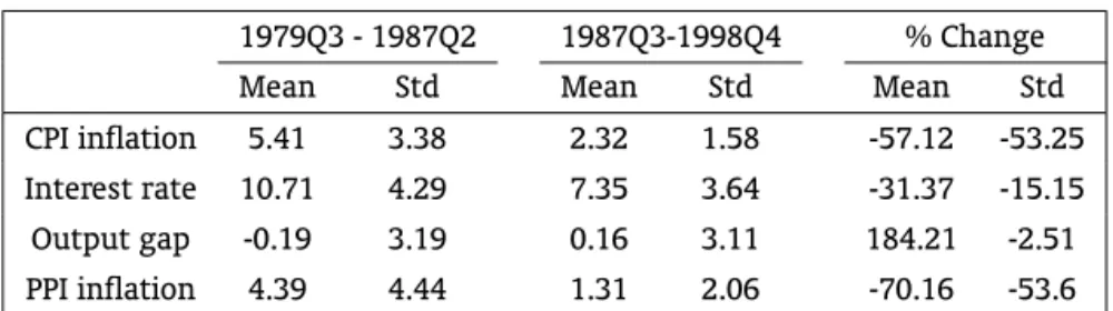
The first subperiod, illustrated in Table 1, is recognized as a high-inflation period and is marked by a turn-over on monetary policies. By the late 80’s, several countries moved to strictly anti-inflation policy rules. Essentially, the economic environment was characterized by high instability, due to the second oil shock, the debit crisis in developing countries, US recession, and inflation. The cost of such economic instability was a widespread economic recession.
The second subperiod, starting at 1987Q3, was dominated by lower average and more stable in-flation rates. Table 1 shows that average inin-flation, measured by both CPI and PPI inin-flation, decreased
6The analysis ends in 1998Q4 due to the official take off of the European Monetary System, after which several European
Table 1 –Descriptive Statistics
1979Q3 - 1987Q2 1987Q3-1998Q4 % Change
Mean Std Mean Std Mean Std
CPI inflation 5.41 3.38 2.32 1.58 -57.12 -53.25
Interest rate 10.71 4.29 7.35 3.64 -31.37 -15.15
Output gap -0.19 3.19 0.16 3.11 184.21 -2.51
PPI inflation 4.39 4.44 1.31 2.06 -70.16 -53.6
by more than 50% when compared to the previous period. Those variables are also much more stable in the second period, as suggested by smaller standard deviations. In fact, the PPI inflation standard deviation was reduced by stunning 70.16%.
Inspired by the successful experience of the US economy, monetary policy practices might have converged to an interest rate rule that displays a vigorous response to inflation variations. The empir-ical evidence shown ahead reveals how this potential common policy rule behaves in a cross-country environment.
4.2. Statistical Properties
The starting point of the empirical evidence is to check whether the panel data is stationary. It is performed panel unit root tests proposed by Levin et al. (2002), Im et al. (2003), and a multivariate version of the augmented Dickey and Fuller test, as suggested by Abuaf and Jorion (1990) and Taylor and Sarno (1998).7Shortly, those tests are labelled as LLC, IPS, and MADF, respectively. Among the three,
the IPS is the least restrictive one because it allows for heterogeneity in the first-order autoregressive parameter under the alternative hypothesis. Serial correlation may be present in the residuals, in which case it is eliminated by including an adequate augmented Dickey and Fuller component in the test equation.
The results are reported in Table 2. Each equation includes 4 lags in the augmented term in order to eliminate potential serial correlation. This lag selection is in accordance with the quarterly feature of the data set. The test equations for the LLC and IPS also include deterministic terms listed in Table 2. Those terms were selected in a general to specific modeling strategy, as suggested by Campbell and Perron (1991). Non-rejection of the null in the most restrictive equation indicates the presence of a unit root. The MADF was not included in this modeling strategy because it assumes only fixed effects in the test equation.
One can see from Table 2 that there is no evidence of a unit root in the series under consideration. Except for the IPS test of the output gap during the low-inflation period, all results indicate rejection of the null under the standard 5% significance level. These findings are maintained as evidence of station-arity of all series in the panel of countries. This is in accordance with the assumption of stationstation-arity found in most of the empirical literature on single-country monetary policy rules.
It is well documented that panel data unit root tests have better power than the time series ones. However, a common criticism to panel data tests states that, under the null hypothesis of unit root, they tend to over-reject the null in the presence of a small subset of stationary series in the panel. To overcome this limitation, it was performed new unit root tests for the country-specific time series, pro-posed by Elliott et al. (1996), Perron and Ng (1996), and Ng and Perron (2001), which use GLS detrended
7Taylor and Sarno (1998) have proposed the combined use of the Johansen likelihood ratio (JLR) test and standard unit root
tests. The JLR test, however, has serious computational limitations for panels with relatively largeN, where one may not have
Table 2 –Panel Data Unit Root Tests
1979Q3 - 1987Q2
LLC IPS MADF Lags
CPI inflation -5.1 none -2.73 {1, t} 72.54 4
Interest rate -1.71 none -2.57 {1, t} 77.87 4
Output gap -4.85 none -1.77 {1} 109.43 4
PPI inflation -3.65 {1, t} -3.05 {1, t} 144.58 4
1987Q3-1998Q4
CPI inflation -1.83 {1, t} -2.64 {1, t} 83.36 4
Interest rate -5.03 none -2.68 {1, t} 66.25 4
Output gap -1.95 {1, t} -1.48⋆ {1} 63.9 4
PPI inflation -2.73 {1} -2.84 {1, t} 78.54 4
1979Q3 - 1998Q4
CPI inflation -1.75 {1, t} -2.75 {1, t} 127.96 4
Interest rate -2.9 {1, t} -2.61 {1, t} 83.15 4
Output gap -7.75 none -2.09 {1} 98.29 4
PPI inflation -5.46 {1, t} -3.76 {1, t} 162.36 4
Note:⋆indicates that the null of unit root is not rejected at 95% confidence level.
data and the modified Akaike information criteria. These tests do not suffer from size and power distor-tions as the traditional ADF and Phillips-Perron unit root tests. The results indicated that the individual time series are stationary and so confirmed the stationarity of the panel of countries.8
4.3. Cross-Country Interest Rate Rules
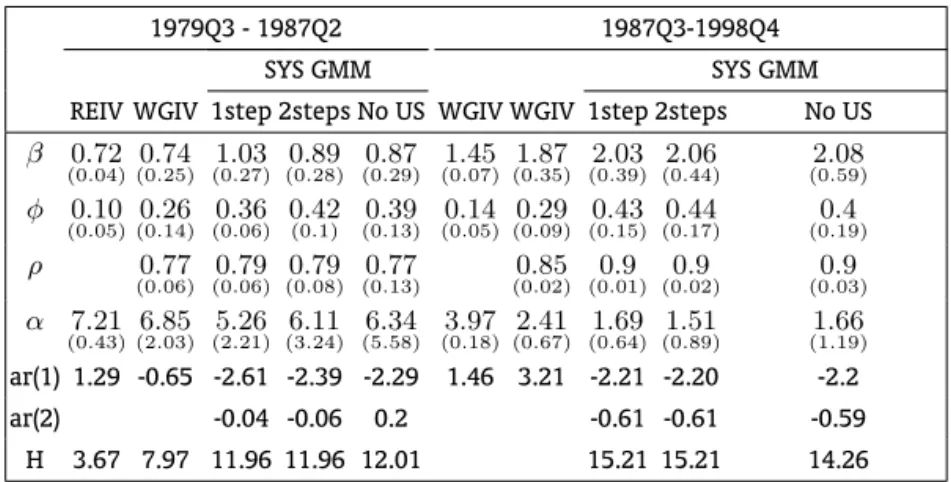
The results for the CPI inflation target case are reported in Table 3. The preferred estimation is given by the two-steps SYS GMM estimator, proposed by Arellano and Bover (1995) and Blundell and Bond (1998). As mentioned before, it provides significant improvements over the original Arellano and Bond (1991) first-differenced GMM estimator. Table 3 also displays results for the one-step SYS GMM and WG IV estimators, which serve the purpose of robustness analyses.
The results indicate that central banks of the selected OECD countries have followed a strict anti-inflation monetary policy in the post-87Q3 period. The coefficient on CPI anti-inflation is significantly greater than one and on output gap is close to 0.5, as suggested by Taylor (1993). There is, however, a consider-able interest rate smoothing, as captured by a first-order autoregressive term of 0.9. Thus, only about 10% adjustment to deviations from the target interest rate occurs within the period of the change.9
The diagnostic tests suggest that the model is well specified, since there is no evidence of second-order residual serial correlation in the first-differenced residuals and the validity of the overidentifying restrictions can not be rejected by the Hansen’sJtest.
8The time series results are not shown to save space but are available upon request.
9Rudebusch (2002) argues that, for the US economy, partial adjustment of the nominal interest rate may, in fact, reflect
Table 3 –Reaction Functions for CPI Inflation Target
1979Q3 - 1987Q2 1987Q3-1998Q4
SYS GMM SYS GMM
REIV WGIV 1step 2steps No US WGIV WGIV 1step 2steps No US
β 0.72
(0.04)
0.74
(0.25)
1.03
(0.27)
0.89
(0.28)
0.87
(0.29)
1.45
(0.07)
1.87
(0.35)
2.03
(0.39)
2.06
(0.44)
2.08
(0.59) φ 0.10
(0.05)
0.26
(0.14)
0.36
(0.06)
0.42
(0.1)
0.39
(0.13)
0.14
(0.05)
0.29
(0.09)
0.43
(0.15)
0.44
(0.17)
0.4
(0.19)
ρ 0.77
(0.06)
0.79
(0.06)
0.79
(0.08)
0.77
(0.13)
0.85
(0.02)
0.9
(0.01)
0.9
(0.02)
0.9
(0.03) α 7.21
(0.43)
6.85
(2.03)
5.26
(2.21)
6.11
(3.24)
6.34
(5.58)
3.97
(0.18)
2.41
(0.67)
1.69
(0.64)
1.51
(0.89)
1.66
(1.19)
ar(1) 1.29 -0.65 -2.61 -2.39 -2.29 1.46 3.21 -2.21 -2.20 -2.2 ar(2) -0.04 -0.06 0.2 -0.61 -0.61 -0.59
H 3.67 7.97 11.96 11.96 12.01 15.21 15.21 14.26
Notes: Standard deviations are reported in parenthesis. For the SYS GMM estimators, the numbers refer to robust standard deviations, using the finite-sample correction for the covariance matrix proposed by Windmeijer (2000).
The serial correlation tests are the Durbin-Watson, for Equation 4, the modified Breusch-Godfrey test, for the WG IV estimator of Equation 3, and them1andm2Arellano and Bond (1991) tests, for the SYS GMM estimator. Notice that negative first-order serial correlation is expected in the first-differenced residuals if the level residuals are uncorrelated. The identifying assumption requires only no second-order serial correlation in the first-differenced residuals (Arellano and Bond, 1991).
For equation (4), Breusch and Pagan (1980) and Hausman (1978) tests were applied to choose the model specification.
As standard instruments, for all estimators, were used lagged values of the variables. The instrument matrix for the SYS GMM estimator includes all variables lagged at t-2 and earlier periods as instruments for the first difference equations and the first differences lagged at t-1 as instruments for the level equations.
As stressed before, the identification strategy pursued here assumes thatπ∗is known and looks for
the value ofr∗ that matches the estimation of the constant term.10 It is assumed a 2% annual rate
for the target inflation in the post-87Q3 period. This implies an equilibrium real interest rate of 3.6%, which is close to the 4% steady state rate usually found in theoretical models. Compared to theex-post
average real interest rate, that value is slightly lower than the 5% derived from Table 1.
The robustness of the previous results is verified by taking US out from the panel of countries, comparing alternative estimation procedures, and relaxing the assumption of partial adjustment. The strictly anti-inflation feature of the monetary policy is still evident in all cases, as the CPI inflation coefficient remains significantly greater than unit. Notice that, for the non-inertial case, the coefficient on inflation rate is statistically greater than one and nearly equal to the 1.5 proposed by Taylor (1993) for the US economy. Using the same identification strategy, the 2% target inflation is coherent with a 4.9% equilibrium real rate, which is virtually identical to theex-post5% derived from Table 1.
Considering the first period, which spans from 1979Q3 to 1987Q2 and is characterized by higher levels of inflation, the previous results do not hold. The two-steps SYS GMM estimator shows that the monetary policy was markedly accommodative, as the estimated CPI inflation coefficient is unit. These findings are supported by diagnostic tests, which indicate that the model is well specified. The
10The assumption of time-invariant common inflation targeting across the major OECD countries is required because the dynamic
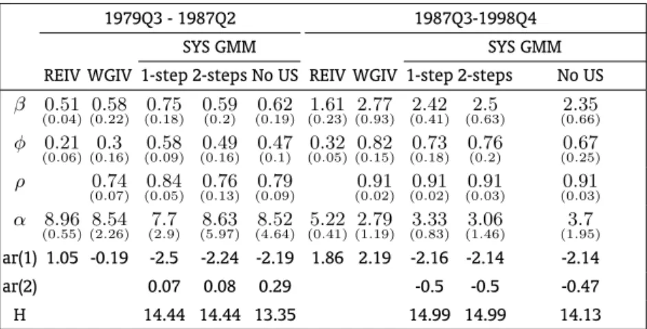
Table 4 –Reaction Functions for PPI Inflation Target
1979Q3 - 1987Q2 1987Q3-1998Q4
SYS GMM SYS GMM
REIV WGIV 1-step 2-steps No US REIV WGIV 1-step 2-steps No US
β 0.51
(0.04)
0.58
(0.22)
0.75
(0.18)
0.59
(0.2)
0.62
(0.19)
1.61
(0.23)
2.77
(0.93)
2.42
(0.41)
2.5
(0.63)
2.35
(0.66) φ 0.21
(0.06)
0.3
(0.16)
0.58
(0.09)
0.49
(0.16)
0.47
(0.1)
0.32
(0.05)
0.82
(0.15)
0.73
(0.18)
0.76
(0.2)
0.67
(0.25)
ρ 0.74
(0.07)
0.84
(0.05)
0.76
(0.13)
0.79
(0.09)
0.91
(0.02)
0.91
(0.02)
0.91
(0.03)
0.91
(0.03) α 8.96
(0.55)
8.54
(2.26)
7.7
(2.9)
8.63
(5.97)
8.52
(4.64)
5.22
(0.41)
2.79
(1.19)
3.33
(0.83)
3.06
(1.46)
3.7
(1.95)
ar(1) 1.05 -0.19 -2.5 -2.24 -2.19 1.86 2.19 -2.16 -2.14 -2.14 ar(2) 0.07 0.08 0.29 -0.5 -0.5 -0.47 H 14.44 14.44 13.35 14.99 14.99 14.13
Notes: Standard deviations are reported in parenthesis. For the SYS GMM estimators, the numbers refer to robust standard deviations, using the finite-sample correction for the covariance matrix proposed by Windmeijer (2000).
The serial correlation tests are the Durbin-Watson, for Equation 4, the modified Breusch-Godfrey test, for the WG IV estimator of Equation 3, and the m1 and m2 Arellano and Bond (1991) tests, for the SYS GMM estimator. Notice that negative first-order serial correlation is expected in the first-differenced residuals if the level residuals are uncorrelated. The identifying assumption requires only no second-order serial correlation in the first-differenced residuals (Arellano and Bond, 1991).
The last row tests the null of valid overidentified restrictions. For the WG estimator it refers to the Haus-man (1978) test, which follows aχ2LwhereLis the number of overidentifying restrictions. For the SYS GMM estimators, the test is the Hansen (1982)Jstatistic. In both cases, the null that the overidentifying restrictions are valid is not rejected.
For equation (4), Breusch and Pagan (1980) and Hausman (1978) tests were applied to choose the model specification.
As standard instruments, for all estimators, were used lagged values of the variables. The instrument matrix for the SYS GMM estimator includes all variables lagged att−2and earlier periods as instru-ments for the first difference equations and the first differences lagged att−1as instruments for the level equations.
sensitivity analysis is also in line with this conclusion as it finds CPI inflation coefficients statistically not different from one in all estimated models.
Turning now to the PPI inflation target case, the evidence of convergence to a strict anti-inflation policy in the recent period is even more convincing. The results displayed in Table 4 show that the PPI inflation coefficient is also significantly greater than one. It is greater than the one found in the CPI inflation target counterpart, but not at reasonable levels of significance.
According to the sensitivity analysis, these findings do not depend on either the presence of the US in the panel of countries, the specific two-steps SYS GMM estimator or the assumption of interest rate smoothness. The last five columns of Table 4 unanimously point out the anti-inflation feature of the monetary policy in the post-87Q3 period. It is interesting to notice that there is no evidence of serial correlation in the non-inertial rule. Thus, the partial adjustment model indeed reflects interest rate smoothness by the OECD central banks.
Applying the same identification strategy as in the case of CPI target, a 2% annual target rate for PPI inflation is coherent with 6% equilibrium real interest rate. Incidentally, this value is identical to the 6%ex-postaverage real rate computed from Table 1. Thus, the PPI inflation target has fit very well the data during the stable inflation period.
both the one-step SYS GMM and the WG IV estimators. As in the CPI inflation target case, there is also a smaller interest rate inertia. About 25% of deviation from the target level is accounted for within the respective period of the shock.
This evidence, however, does not mean that the monetary policy was destabilizing in the first pe-riod. It indicates that a Taylor-type of interest rate rule that uses PPI as measure of inflation was not suited to describe a common monetary policy in the first period. Nevertheless, after 1987Q3 the major OECD central banks have moved to an explicit anti-inflation interest rate rule, as identified by both the CPI and PPI targeting regimes. This result suggests a convergence of monetary policy practices among the selected OECD countries.
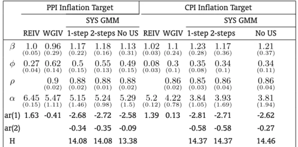
The change of regime is confirmed by the results reported in Table 5, which displays estimations for the whole period. One can see that, under both targeting regimes, the interest rate rule displays coef-ficients on inflation that are statistically not different from one. This evidence is robust to alternative estimation procedures and to the exclusion of the US from the panel of countries. Thus, there has been indeed a change of behavior towards a strict anti-inflation interest rate rule in the post-87Q3 period.
Table 5 –Estimated Reaction Functions for the Whole Period: 1979Q3 to 1998Q4
PPI Inflation Target CPI Inflation Target
SYS GMM SYS GMM
REIV WGIV 1-step 2-steps No US REIV WGIV 1-step 2-steps No US
β 1.0
(0.05)
0.96
(0.29)
1.17
(0.22)
1.18
(0.16)
1.13
(0.31)
1.02
(0.03)
1.1
(0.24)
1.23
(0.28)
1.17
(0.36)
1.21
(0.37) φ 0.27
(0.04)
0.62
(0.14)
0.5
(0.15)
0.55
(0.13)
0.49
(0.15)
0.08
(0.03)
0.3
(0.1)
0.35
(0.08)
0.34
(0.1)
0.34
(0.11)
ρ 0.9
(0.02)
0.88
(0.02)
0.88
(0.01)
0.88
(0.02)
0.86
(0.02)
0.85
(0.03)
0.86
(0.04)
0.86
(0.04) α 6.45
(0.15)
5.47
(1.11)
5.15
(1.46)
5.24
(0.98)
5.29
(1.5)
5.2
(0.12)
4.22
(0.78)
3.84
(1.05)
3.93
(1.69)
3.81
(1.94)
ar(1) 1.63 -0.41 -2.68 -2.72 -2.58 1.39 0.13 -2.81 -2.71 -2.62 ar(2) -0.34 -0.35 -0.09 -0.58 -0.58 -0.27 H 14.08 14.08 13.38 14.37 14.37 14.46
Notes: Standard deviations are reported in parenthesis. For the SYS GMM estimators, the numbers refer to robust standard deviations, using the finite-sample correction for the covariance matrix proposed by Windmeijer (2000).
The serial correlation tests are the Durbin-Watson, for Equation 4, the modified Breusch-Godfrey test, for the WG IV estimator of Equation 3, and the m1 and m2 Arellano and Bond (1991) tests, for the SYS GMM estimator. Notice that negative first-order serial correlation is expected in the first-differenced residuals if the level residuals are uncorrelated. The identifying assumption requires only no second-order serial correlation in the first-differenced residuals (Arellano and Bond, 1991).
The last row tests the null of valid overidentified restrictions. For the WG estimator it refers to the Haus-man (1978) test, which follows aχ2
LwhereLis the number of overidentifying restrictions. For the SYS
GMM estimators, the test is the Hansen (1982)Jstatistic. In both cases, the null that the overidentifying restrictions are valid is not rejected.
For equation (4), Breusch and Pagan (1980) and Hausman (1978) tests were applied to choose the model specification.
As standard instruments, for all estimators, were used lagged values of the variables. The instrument matrix for the SYS GMM estimator includes all variables lagged att−2and earlier periods as instruments for the first difference equations and the first differences lagged att−1as instruments for the level equations.
5. CONCLUSION
sixteen major OECD countries during the period 1979Q2 to 1998Q4. Under the influence of the United States monetary policy, the sample was divided into two subperiods, with 87Q3 being the breaking point. Cross-country reaction functions were estimated using two alternative measures of inflation, represented by CPI and PPI annualized rates.
The results pointed to a convergence of monetary policy practices among the selected OECD coun-tries in the post-87Q3 period. The cross-country interest rate rule displayed coefficient on inflation rate that is statistically greater than one. On the other hand, during the period 79Q3 to 87Q2, there is evi-dence of a accommodative monetary policy. The response of the nominal interest rate to CPI inflation variations was statisticaly not different from one. This last result also holds if one considers estimations for the whole period.
Sensitivity analyses showed that the previous results do not depend on either the presence of US in the panel of countries, the specific system GMM estimator or the assumption of interest rate smoothing. In fact, the static version of the policy rule adjusted very well to the panel data according to diagnostic tests. For instance, it did not display the highly serially correlated residuals that is usually found in single-country estimations. Hence, the cross-country partial adjustment model reflects an interest rate smoothing behavior by the selected central banks.
Comparing performances of alternative measures of inflation, it is fair to state that the PPI inflation has also played an implicit role of targeting rate in the latter period. The estimated reaction functions displayed an aggressive inflation-stabilization policy in well specified models. In addition, the identified equilibrium real interest rate exactly matched the actual ex-postreal interest rate. This finding is in agreement with the theoretical result that monetary authority should target PPI inflation in a typical small open economy.
BIBLIOGRAPHY
Abuaf, N. & Jorion, P. (1990). Purchasing power parity in the long run.Journal of Finance, 45:157–174.
Arellano, M. & Bond, S. (1991). Some tests of specification for panel data: Monte Carlo evidence and an application to employment equations. Review of Economic Studies, 58:277–297.
Arellano, M. & Bover, O. (1995). Another look at the instrumental variable estimation of error-components models. Journal of Econometrics, 68:29–51.
Blundell, R. & Bond, S. (1997). Initial conditions and moment restrictions in dynamic panel data models.
Journal of Econometrics, 87:115–143.
Blundell, R. & Bond, S. (1998). GMM estimation with persistent panel data: An application to production functions. Technical Report CWP99/4, Institute for Fiscal Studies.
Breusch, T. & Pagan, A. (1980). The LM test and its applications to model specification in econometrics.
Review of Economics Studies, 47:239–254.
Campbell, J. Y. & Perron, P. (1991). Pitfalls and opportunities: What macroeconomists should know about unit roots. NBER Technical Working Papers 0100, National Bureau of Economic Research, Inc.
Clarida, R., Gali, J., & Gertler, M. (1998). Monetary policy rules in practice some international evidence.
European Economic Review, 42:1033–1067.
Clarida, R., Gali, J., & Gertler, M. (2000). Monetary policy rules and macroeconomic stability: Evidence and some theory. Quarterly Journal of Economics, 115:147–180.
Divino, J. A. (2009). Optimal monetary policy for a small open economy.Economic Modelling, 26:352–58.
Doyle, M. & Falk, B. (2008). Testing commitment models of monetary policy: Evidence from OECD economies. Journal of Money, Credit and Banking, 40:409–25.
Elliott, G., Rothenberg, T. J., & Stock, J. H. (1996). Efficient tests for an autoregressive unit root. Econo-metrica, 64:813–36.
Gali, J. & Monacelli, T. (2005). Monetary policy and exchange rate volatility in a small open economy.
Review of Economic Studies, 72:707–734.
Hansen, L. (1982). Large sample properties of generalized method of moments estimators.Econometrica, 50:1029–1054.
Hausman, J. (1978). Specification tests in econometrics.Econometrica, 46:1251–1271.
Im, K., Pesaran, M., & Shin, Y. (2003). Testing for unit roots in heterogeneous panels. Journal of Econo-metrics, 115:53–74.
Judd, J. & Rudebusch, G. (1998). Taylor’s rule and the Fed: 1970–1997. Federal Reserve Bank of San Francisco Economic Review, 3:3–16.
Levin, A., Lin, C., & Shu, C. (2002). Unit root tests in panel data: Asymptotic and finite-sample properties.
Journal of Econometrics, 108:1–24.
Ng, S. & Perron, P. (2001). Lag length selection and the construction of unit root test with good size and power.Econometrica, 69:1519–54.
Perron, P. & Ng, S. (1996). Useful modifications to unit root tests with dependent errors and their local asymptotic properties. Review of Economic Studies, 63:435–65.
Rudebusch, G. (2002). Term structure evidence on interest rate smoothing and monetary policy inertia.
Journal of Monetary Economics, 49:1161–1187.
Taylor, J. B. (1993). Discretion versus policy rules in practice. Carnegie-Rochester Series on Public Policy, 39:195–214.
Taylor, M. & Sarno, L. (1998). The behavior of real exchange rates during the post-bretton woods period.
Journal of International Economics, 46:281–312.
Wang, P. & Wen, Y. (2007). Inflation dynamics: A cross-country investigation. Journal of Monetary Economics, 54:2004–31.
Windmeijer, F. (2000). A finite sample correction for the variance of linear two-step GMM estimators. Technical Report CWP00/19, Institute for Fiscal Studies.
Woodford, M. (2003). Interest Rate and Prices: Foundations of a Theory of Monetary Policy. Princeton University Press, Princeton.