Haplotyping a quantitative trait with a high-density map in experimental crosses.

(1)

Haplotyping a Quantitative Trait with a High-Density

Map in Experimental Crosses

Wei Hou1, John Stephen F. Yap2, Song Wu2, Tian Liu2, James M. Cheverud3, Rongling Wu2*

1Department of Epidemiology and Health Policy Research, University of Florida, Gainesville, Florida, United States of America,2Department of Statistics, University of Florida, Gainesville, Florida, United States of America,3Department of Anatomy and Neurobiology, Washington University Medical School, St. Louis, Missouri, United States of America

Background.The ultimate goal of genetic mapping of quantitative trait loci (QTL) is the positional cloning of genes involved in any agriculturally or medically important phenotype. However, only a small portion (#1%) of the QTL detected have been characterized at the molecular level, despite the report of hundreds of thousands of QTL for different traits and populations. Methods/Results.We develop a statistical model for detecting and characterizing the nucleotide structure and organization of haplotypes that underlie QTL responsible for a quantitative trait in an F2pedigree. The discovery of such haplotypes by the

new model will facilitate the molecular cloning of a QTL. Our model is founded on population genetic properties of genes that are segregating in a pedigree, constructed with the mixture-based maximum likelihood context and implemented with the EM algorithm. The closed forms have been derived to estimate the linkage and linkage disequilibria among different molecular markers, such as single nucleotide polymorphisms, and quantitative genetic effects of haplotypes constructed by non-alleles of these markers. Results from the analysis of a real example in mouse have validated the usefulness and utilization of the model proposed.Conclusion.The model is flexible to be extended to model a complex network of genetic regulation that includes the interactions between different haplotypes and between haplotypes and environments.

Citation: Hou W, Yap JSF, Wu S, Liu T, Cheverud JM, et al (2007) Haplotyping a Quantitative Trait with a High-Density Map in Experimental Crosses. PLoS ONE 2(8): e732. doi:10.1371/journal.pone.0000732

INTRODUCTION

The basic principle for quantitative trait locus (QTL) mapping is the cosegregation of the alleles at a QTL with those at one or a set of known polymorphic markers genotyped on a genome in an experimental cross [1,2]. If a QTL is cosegregating with molecular markers, the genetic effects of the QTL on a quantitative trait and its genomic position can be estimated from the marker genotypes and phenotypic values of the trait. This estimation process particularly assumes the QTL to be located within an interval constructed by a pair of flanking markers in which a test statistics calculated under the reduced (there is no QTL) and full model (there is a QTL) is used to test the existence of the QTL and estimate its position. This so-called interval mapping approach and its extensions [3–5] is robust and powerful for the detection of major QTL and presents the most efficient way to utilize marker information when marker maps are sparse [6]. However, interval mapping is limited by its incapacity to infer any information about the sequence structure and organization of the QTL. Partly for this reason, only a few QTL mapped from markers have been successfully cloned [7–9], despite a considerable number of QTL reported in the literature.

Interval QTL mapping also has an unsolved statistical difficulty when it is used with a high-density linkage map. With more markers genotyped, a genetic map for QTL identification has tended to be infinitely dense. For such an infinitely dense map in which markers are located everywhere over the genome, test statistics at nearby intervals are not independent any more. Thus, the critical threshold used to acclaim the existence of a QTL by interval mapping will be difficult to analytically determine. Although an empirical alternative based on permutation tests has been proposed for threshold determination [10], extensive computing may affect the use efficiency of interval mapping.

Despite its unsuitability for interval mapping of QTL, an infinitely dense map provides an important tool for characterizing genetic variants that contribute to quantitative variation via the analysis of haplotypes composed of non-alleles at a set of highly

linked markers. Recent genetic studies suggest that a gene may determine a complex trait, such as body weight or drug response, through its haplotype rather than genotype [11,12]. The completion of the genome projects for several important organ-isms, Arabdopsis, chicken, human, mouse and poplar, has made massive amounts of DNA sequence data available. In particular, single nucleotide polymorphisms (SNPs), being the most common type of variant in the DNA sequence, provide a powerful means for genotyping the whole genome or any part of it. This facilitates the identification of specific SNP-constructed haplotypes which are responsible for quantitative traits. A set of SNPs that cause quantitative differences among individuals are called quantitative trait nucleotides (QTNs). Liu et al. [13] proposed a statistical model for estimating and testing haplotype effects at a QTN in a random sample drawn from a natural population. This model is based on the population genetic properties of gene segregation. Through the implementation of the EM algorithm, population genetic parameters of SNPs, such as haplotype frequencies, allele frequencies and linkage disequilibria, and quantitative genetic parameters, such as haplotype effects of a QTN, are estimated with closed forms.

Academic Editor:Peter Heutink, Vrije Universiteit Medical Centre, Netherlands

ReceivedApril 10, 2007;AcceptedJuly 13, 2007;PublishedAugust 15, 2007

Copyright:ß2007 Hou et al. This is an open-access article distributed under the terms of the Creative Commons Attribution License, which permits unrestricted use, distribution, and reproduction in any medium, provided the original author and source are credited.

Funding:The preparation of this manuscript is supported by NSF grant (0540745) to RW.

Competing Interests:The authors have declared that no competing interests exist.

(2)

The motivation of this work is to derive a statistical model for haplotype discovery responsible for quantitative variation in a mapping population derived an experimental cross. Unlike a natural population in which gene co-segregation analysis is based on linkage disequilibria [14], experimental crosses, such as the backcross or F2, have usually been analyzed in terms of the linkage between different markers and QTL. In this article, we will frame a general statistical model for estimating the linkage between different SNPs and testing haplotype effects within the context of linkage disequilibrium analysis in an F2pedigree. We show that the new model can test for the dependence of SNPs when a multi-point analysis is performed. We have derived closed forms for the EM algorithm to estimate a variety of genetic parameters. A worked example is used to validate the usefulness and utilization of the model.

METHODS

Haplotype and diplotype

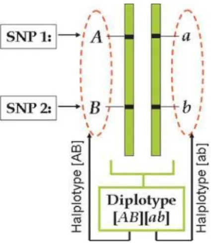
A haplotype represents a linear arrangement of nucleotides (alleles) at different SNPs on a single chromosome, or part of a chromosome. The pair of haplotypes is called a diplotype. The observed phenotype of a diplotype is called a genotype. A diplotype is always constructed by two haplotypes, one from the maternal parent and the other from the paternal parent. Suppose there are two different SNPs on the same genomic region, one with two allelesAandaand the other with two allelesBandb, respectively. AlleleAfrom SNP 1 and alleleBfrom SNP 2 are located on the first homologous chromosome, whereas allele

afrom SNP 1 and allele bfrom SNP 2 located on the second homologous chromosome. Thus, [AB] is one haplotype and [ab] is a second haplotype, and both constitute a diplotype [AB][ab] (Fig. 1).

In a practical genetic analysis, we can only observe the genotype expressed asAa/Bb. However, the double heterozygote may be one (and only one) of two possible diplotypes [AB][ab] and [Ab][aB]. But these two diplotypes cannot be directly observed and should be inferred from SNP genotype data (Fig. 2). In practice, it is important to estimate haplotype effects on a quantitative trait based on the diplotypes and therefore genotypes. For example, if an animal carries haplotype [AB], it will grow better than other animals that carries any other haplotypes, [Ab], [aB] and [ab]. For this reason, the same

genotype Aa/Bb may perform differently, depending on what diplotype it carries. If this genotype is diplotype [AB][ab], then it will have a better growth. If the animal is diplotype [Ab][aB], its growth will be poorer. The statistical model being developed will be used to determine which diplotype is associated with better growth in experimental crosses.

Linkage disequilibrium in the F

2

intercross

A general model: Haplotype analysis in the backcross is straightforward because the diplotype is determined for all the backcross genotype. Simple analysis of variance can be used to detect haplotype effects on a quantitative trait. In the F2, this is not a case in which the double heterozygote is a mixture of two possible diplotypes.

Suppose many SNPs are genotyped each of which is segregating in a 1:2:1 Mendelian ratio in the F2 population. As seen in the human genome [15], these SNPs are divided into different haplotype blocks. For a given block, there are a particular number of representative SNPs or htSNPs that uniquely identify the common haplotypes in this block or QTN. Several algorithms have been developed to identify a minimal subset of htSNPs that can characterize the most common haplotypes [16–18]. Consider a QTN that contains L htSNPs among which there exist linkage disequilibria of different orders. The two alleles, 1 and 0, at each of these SNPs are symbolized by r1,…,rL, respectively. For a cross initiated with two inbred parents, the allele frequencies for each of these htSNPs should be 1/2. A haplotype frequency, denoted aspr1r2rL, is decomposed into the following components:

pr1r2...rL

~pr1pr2. . .prL No LD

z({1)rL{1zrL_p

r1. . .prL{2D(L{1)Lz. . .

z({1)r1zr2_p

r3. . .prLD12 Digenic LD

z({1)rL{2zrL{1zrL_p

r1. . .prL{3D(L{2)(L{1)L

z. . .z({1)r1zr2zr3_p

r4. . .prLD123 Trigenic LD

z. . .

z({1)L₍_{₁₎r1z...zrL_D

1...L Lgenic LD ð1_Þ

whereD’s are the linkage disequilibria of different orders among particular SNPs.

Figure 1. Haplotype configuration of a diplotype for two hypothe-sized SNPs.

doi:10.1371/journal.pone.0000732.g001

Figure 2. Diplotype configuration of a genotype for two hypothe-sized SNPs.

(3)

Totally, L SNPs form 2L haplotypes expressed as [r1…rL], 2L21(2L+1) diplotypes, i.e., a pair of maternally- (m) and paternally-derived haplotypes (p), expressed as [r1m…rLm] [r1

p …rL

p ] (r1

m , r1

p ,…;rL

m ,rL

p

= 1,0) and 3L genotypes expressed as r1r91/…/rLr9L (r1$r91,…,rL$r9L=1,0). Only genotypes can be observed. The number of diplotypes is smaller than the number of genotypes because the genotypes that are heterozygous at two or more SNPs contain multiple different diplotypes. Diplotype (and therefore genotype) frequencies can be expressed in terms of haplotype frequencies. We useP_½rm

1:::r m

L½r

p 1:::r

p

LandPr1r01=...=rLr0L to denote the diplotype and genotype frequencies, respectively, and nr1r01=...=rLr0L to denote genotype observation.

A special case: Two-point linkage disequilibrium:For two given SNPs (S1andS2), there are four different haplotypes in a cross population. According to the definition given above, these four haplotypes are denoted as [11], [10], [01] and [00], whose frequencies in a cross population are, respectively, expressed as

p11~

1 4zD,

p10~

1 4{D,

p01~

1 4{D,

p00~

1 4zD:

ð2Þ

Assume that the two SNPs are linked with a recombination fractionr. The haplotype frequencies can be expressed in terms of

r, i.e., p11~

1

2(1{r), p10~ 1 2r, p01~

1

2r and p00~ 1

2(1{r). Com-bining equation (2), this establishes the relation between the linkage disequilibrium and recombination fraction as

D~1

4(1{2r), ð3Þ

or

r~1

2(1{4D): ð4Þ

A special case: Three-point linkage disequilibrium: For three given SNPs (S1, S2, and S3), there are eight different haplotypes, i.e., [111], [110], [101], [100], [011], [010], [001], and [000]. The haplotype frequencies in a cross population are, respectively, expressed as

p111~

1 8z

1 2D23z

1 2D13z

1

2D12zD123 p110~

1 8{

1 2D23{

1 2D13z

1

2D12{D123 p101~

1 8{

1 2D23z

1 2D13{

1

2D12{D123 p100~

1 8z

1 2D23{

1 2D13{

1

2D12zD123 p011~

1 8z

1 2D23{

1 2D13{

1

2D12{D123 p010~

1 8{

1 2D23z

1 2D13{

1

2D12zD123 p001~

1 8{

1 2D23{

1 2D13z

1

2D12zD123 p000~

1 8z

1 2D23z

1 2D13z

1

2D12{D123

ð5Þ

whereD12,D23andD13are the linkage disequilibria between SNP

S1andS2, betweenS2andS3and betweenS1andS2, respectively, andD123is the linkage disequilibrium among the three SNPs. The four disequilibrium coefficients can be estimated, by solving equation (5), as

D12 ~ 1

4½(p111zp110zp001zp000){(p101zp100zp011zp010)

D23 ~ 1

4½(p111zp011zp100zp000){(p110zp010zp101zp001)

D13 ~ 1

4½(p111zp101zp010zp000){(p110zp100zp011zp001)

D123 ~ 1

8½(p111zp100zp010zp001){(p110zp101zp011zp000)

ð6Þ

The first three first-order linkage disequilibria can be used to describe the linkage between different SNPs and crossover interference, whereas the last second-order linkage disequilibrium is thought to be associated with chromatid interference.

Haplotyping a trait with two SNPs

Our interest is to search for the haplotype diversity that can explain phenotypic variation in a complex trait. The association between haplotype diversity and phenotypic variation has been detected in several studies of drug responses [11,12]. This allows us to assume that a particular haplotype is different from other haplotypes for a given trait. Here, our focus will be on modelling haplotype effects in experimental crosses. Although haplotypes (comprising diplotypes) can be directly observed in the backcross, this is not possible for the F2because their heterozygous genotypes are not concordant with diplotypes or haplotypes. For the F2 population, the effects of different haplotypes on the phenotype need be postulated from observed zygotic genotypes. The inference of diplotypes for a particular genotype is statistically a missing data problem that can be formulated by a finite mixture model.

Mixture model:The statistical method for the genomewide scan of QTN is formulated on the basis of a finite mixture model. The mixture model assumes that each observation comes from one of an assumed set of distributions. The mixture model derived to detect haplotype effects on a quantitative trait based on SNP genotype data contains three major parts: (1) the mixture proportions of each distribution, denoted as the relative frequen-cies of different diplotypes for the same SNP genotype, (2) the mean for each diplotype in the density function, and (3) the residual variance common to all diplotypes.

For simplicity, we consider a QTN that is composed of only two SNPs each with two alleles designated as 1 and 0. These two SNPs segregating in the F2 population form four haplotypes whose frequencies are arrayed in vectorHp = (p11, p10, p01, p00). All the genotypes are consistent with diplotypes, except for the double heterozygote, 10/10, that contains two different diplotypes [11][00] with a frequency of 2p11p00and [10][01] with a frequency of 2 p10p01 (Table 1). The relative frequencies of different diplotypes for the double heterozygote are a function of haplotype frequencies.

A total ofnindividuals in the F2are classified into 9 genotypes for the two SNPs, each genotype with observation generally expressed asnr1r01=r2r02 (r1$r91,r2$r92,r3$r93= 1,0). The frequency

(4)

of the trait (yi) for individualiis expressed by a linear model, i.e.,

yi~ X1

rm 1~0

X1

rp1~0

X1

rm 2~0

X1

rp2~0 jiu_½rm

1r m 2½r

p 1r

p 2

zei, ð7Þ

where ji is the indicator variable defined as 1 if a diplotype considered is compatible with subject i and as 0 otherwise, u_½rm

1r m 2½r

p 1r

p 2

~u_½rp₁rp₂½rm 1r

m

2 is the genotypic value for diplotype

½rm₁rm₂½rp₁rp₂, andeiis the residual error distributed asN(0,s2). Assume that this QTN triggers an effect on the trait because at least one haplotype is different from the remaining seven. Without loss of generality, let [11] be such a distinct haplotype, calledrisk haplotype, designated asA. All the other non-risk haplotypes, [10], [01] and [00], are collectively expressed asA¯. The risk and non-risk haplotypes form threecomposite diplotypes AA(2),AA¯(1) andA¯A¯

(0). Letm2,m1andm0be the genotypic value of the three composite diplotypes, respectively (Table 1). The means for different composite diplotypes and residual variance are arrayed by a quantitative genetic parameter vectorHq= (m2,m1,m0,s

2

). Likelihoods: With the above notation, we construct two likelihoods, one for haplotype frequencies (Hp) based on SNP data (S) and the other for quantitative genetic parameters (Hq) based on haplotype frequencies (Hp), phenotypic (y) and SNP data (S). They are, respectively, expressed as

logL(HpjS)~ logL(HpjHq,y,S)~

z2n11=11logp11 P

n11=11

i~1

logf2(yi)

zn11=10log (2p11p10) zP

n11=10

i~1 logf1(yi) z2n11=00logp10 z

Pn11=00

i~1 logf0(yi) zn10=11log (2p11p01) zP_i~n10=₁11logf1(yi) zn10=10log (2p11p00z2p10p01) zP

n10=10

i~1 log½wf1(yi)z(1{w)f0(yi) zn10=00log (2p10p00) zP_i~n10=₁00logf0(yi)

z2n00=11logp01 zP

n00=11

i~1 logf0(yi) zn00=10log (2p01p00) zP_i~n00=₁10logf0(yi)

z2n00=00logp00 zP

n00=00

i~1 logf0(yi) ð8_Þ

wherefj(yi) is a normal distribution density function of composite diplotypej(j= 2,1,0), i.e.,

fj(yi)~ _{ffiffiffiffiffiffi}1

2p

p

sexp {

(yi{mj)2 2s2

" #

:

It can be seen from the above likelihood functions that, although most zygote genotypes contain a single component (diplotype), the double heterozygote is the mixture of two possible diplotypes weighted bywand 1-w, expressed as

w~ p11p00

p11p00zp10p01

, ð9Þ

which represents the relative frequency of diplotype [11][00] for the double heterozygote.

It should be noted thatL(Hp,Hq|y,S) relies on the haplotype frequencies defined inL(Hp|S) and, thus, the latter is thought to be nested within the former. The estimates of parameters that maximizeL(Hp|S) can also maximize theL(Hp,Hq|y,S).

The EM algorithm: A closed-form solution for the EM algorithm has been derived to estimate the unknown parameters that maximize the two likelihoods of (26) [13]. The estimates of haplotype frequencies are based on the log-likelihood function

L(Hp|M), whereas the estimates of diplotype genotypic means and residual variance are based on the log-likelihood functionL(Hp,Hq |y,M). These two different types of parameters can be estimated using a two-stage hierarchical EM algorithm.

At a higher hierarchy of the EM algorithm, the E step is aimed to calculate the relative frequency (w) of diplotype [11][00] in the double heterozygote is calculated by equation (9). The M step is aimed to estimate the haplotype frequencies based on the probabilities calculated in the previous iteration using

^

p p₁₁~1

2n(2n11=11zwn10=10zn11=10zn10=11)

^

p p10~

1

2n½2n11=00zn11=10z(1{w)n10=10zn10=00

^

p p01~

1

2n½2n00=11zn10=11z(1{w)n10=10zn00=10

^

p p00~

1

2n(2n00=00zwn10=10zn01=00zn10=00)

ð10Þ

Table 1.Diplotypes and their frequencies for each of nine genotypes at two SNPs within a QTN, haplotype composition frequencies for each genotype, and composite diplotypes for four possible risk haplotypes.

. . . .

Genotype Diplotype

Relative diplotype frequency Risk haplotype

Configuration Frequency [11] [10] [01] [00]

11/11 [11][11] p211 1 AA A¯ A¯ A¯ A¯ A¯ A¯

11/10 [11][10] 2p11p10 1 AA¯ AA¯ A¯ A¯ A¯ A¯

11/00 [10][10] p210 1 A¯ A¯ AA A¯ A¯ A¯ A¯

10/11 [11][01] 2p11p01 1 AA¯ A¯ A¯ AA¯ A¯ A¯

10/10 _½11½00

½10½01

2p11p00

2p10p01

w

1{w

AAA A AAA

A AAA AAA

AAA A AAA

10/00 [10][00] 2p10p00 1 A¯ A¯ AA¯ A¯ A¯ AA¯

00/11 [01][01] p201 1 A¯ A¯ A¯ A¯ AA A¯ A¯

00/10 [01][00] 2p01p00 1 A¯ A¯ A¯ A¯ AA¯ AA¯

00/00 [00][00] p200 1 A¯ A¯ A¯ A¯ A¯ A¯ AA

Two alleles for each of the two SNPs are denoted as 1 and 0, respectively. Genotypes at different SNPs are separated by a slash. Diplotypes are the combination of two bracketed maternally and paternally derived haplotypes. By assuming different haplotypes as a risk haplotype, composite diplotypes are accordingly defined and their genotypic values are given.

doi:10.1371/journal.pone.0000732.t001

..

....

...

....

...

....

...

....

...

....

...

....

...

....

(5)

At a lower hierarchy of the EM algorithm, the E step is derived to calculate the posterior probability (V[11][00]i) of individualiwith the double heterozygous genotype to be diplotype [11][00] by

V_½11½00i~

wf_½11½00(yi)

wf_½11½00(yi)z(1{w)f½10½01(yi)

:

Note that for all the other genotypes, such posterior probabilities do not exist.

By assuming that [11] is a risk haplotype, the M step is derived to estimate the genotypic values (mj) for each composite diplotype and the residual variance based on the calculated posterior probabilities by

^

m

m2 ~

Pn₁₁₌₁₁ i~1 yi

n11=11 ,

^

m

m₁ ~

Pnn_

i~1yiz

Pn₁₀₌₁₀ i~1 V½11½00iyi _

n nzPn10=10

i~1 V½11½00i

,

^

m

m0 ~

P€nn i~1yiz

Pn₁₀₌₁₀

i~1 (1{V½11½00i)yi

€

n nzPn10=10

i~1 (1{V½11½00i)

,

ð12Þ

^

s

s2 ~ 1

nf P n11=11

i~1

(yi{mm^2)2zP

_

n n

i~1

(yi{^mm1)2zP

€

n n

i~1

(yi{mm^0)2

z P

n10=10

i~1

V_½10=10i(yi{mm^1)2z(1{V½10=10i)(yi{^mm0)2

g,

ð13Þ

where

_

n

n~n11=10zn10=11,

€

n

n~_n₁₁₌₀₀z_n₁₀₌₀₀z_n₀₁₌₀₁z_n₀₁₌₀₀z_n₀₀₌₀₀:

Iterations including the E and M steps are repeated at the higher hierarchy between equations (9) and (10) and at the lower hierarchy among equations (12) and (13) until the estimates of the parameters converge to stable values. The sampling errors of these parameters can be estimated by calculating Louis’ [19] observed information matrix.

Haplotype frequencies can be expressed as a function of allelic frequencies and linkage disequilibrium. Based on equation (2), we solve the linkage disequilibrium between two SNPs by

^

D D~_^pp11{

1 4

~1

4{^pp10:

ð14Þ

With the genotypic means of composite diplotypes, we can estimate the overall mean (m) and additive (a) and dominant genetic effects (d) due to the QTN detected, respectively, by

^

m

m ~ 1

2(^mm2zmm^0)

^

a

a ~ 1

2(^mm2{mm^0)

^

d

d ~ _^mm1{

1 2(mm^2z^mm0)

Model selection:The likelihoodL(Hp,Hq|y,S) is formulated by assuming that haplotype [11][11] is a risk haplotype. However,

a real risk haplotype is unknown from raw data (y, S). An additional step for the choice of the most likely risk haplotype should be implemented. The simplest way to do so is to calculate the likelihood values by assuming that any one of the four haplotypes can be a risk haplotype (Table 1). Thus, we obtain four possible likelihood values under different risk haplotypes; that is, (1) L1( ^HHp, ^HH1qjy,S) for [11], (2)L2( ^HHp, ^HH2qjy,S) for [10], (3) L3( ^HHp, ^HH3qjy,S) for [01], and (4) L4( ^HHp, ^HH4qjy,S) for [00]. Under each possible risk haplotype, we estimate the quantitative genetic parametersHH^kq (k= 1,…,4). The largest likelihood value calculated is thought to correspond to the most likely risk haplotype.

In practice, it is also possible that there exist more than one risk haplotypes for a QTN. Relative to the bi-‘‘allelic’’ QTN with one risk haplotype, such a QTN is called a multi-‘‘allelic’’ QTN. If there are two risk haplotypes, we will have six composite diplotypes. Assuming that [11] (denoted byA1) and [10] (denoted byA2) are risk haplotypes and the remaining haplotypes [10] and [01] are non-risk haplotypes (denoted byA3), then six composite diplotypes, expressed asA1A1,A1A2, A1A3, A2A2, A2A3 andA3A3, can be specified according to the diplotype distribution as shown in Table 1. Totally, there are six such haplotype combinations for a two-SNP QTL, each combination corresponding to a likelihood value. Based on the calculated likelihoods, we can determine a most likely risk and non-risk haplotype combination. If there are three risk haplotypes, we will have 10 different composite diplotypes. The optimal risk and non-risk haplotype combination will be selected from three combinations based on the likelihoods. The likelihood can be used as a criterion to select the optimal risk and non-risk haplotype combination when the number of risk haplotype is the same. However, when the number of risk haplotype is different, an AIC- or BIC-based model selection strategy [20] should be used because of different numbers of parameters being estimated in this case.

Hypothesis tests:We can test two major hypotheses in the following sequence: (1) the association between two SNPs by testing their linkage disequilibrium, and (2) the difference of a given haplotype from the remaining haplotypes by testing the signifi-cance of haplotype additive and dominant effects on the trait. The linkage disequilibrium between two given SNPs can be tested using two alternative hypotheses:

H0:D~0 vs:H1:D=0

The log-likelihood ratio test statistic for the significance of LD is calculated by comparing the likelihood values under theH1(full model) andH0(reduced model) using

LR1~{2½logL(p11~p10~p01~p00~

1

4jS){logL(HH^pjS), ð16Þ

TheLR1 is considered to asymptotically follow ax2distribution with one degree of freedom.

Diplotype or haplotype effects on the trait, i.e., the existence of a QTN, can be tested using the following hypotheses expressed as

H0:mj:mvs:H1:at least one equality inH0does not hold,j~2,1,0ð17Þ

The log-likelihood ratio test statistic (LR2) under these two hypotheses can be similarly calculated,

(6)

where the tildes and hats denote the MLEs of parameters under the null and alternative hypotheses of (17), respectively. Although the critical threshold for determining the existence of a QTN can be based on empirical permutation tests, theLR2may asymptotically follow a x2

distribution with two degrees of freedom, so that the threshold can be obtained from the x2 distribution table.

Haplotyping a trait with multiple SNPs

Haplotype structure: The statistical method for QTN mapping is exemplified by a set of three SNPs, S1–S3, for a QTN. Two alleles 1 and 0 at each SNP are symbolized byr1, r2 and r3, respectively. Eight haplotypes, [111], [110], [101], [100], [011], [010], [001] and [000], formed by these three SNPs, have the frequencies arrayed inHp= (p111,p110,p101,p100, p011, p010, p001, p000). Some genotypes are consistent with diplotypes, whereas the others that are heterozygous at two or more SNPs are not. Each double heterozygote contains two different diplotypes. One triple heterozygote, i.e., 10/10/10, contains four different diplotypes, [111][000] (in a probability of 2p111p000), [110][001] (in a probability of 2p110p001), [101][010] (in a probability of 2p101p010) and [100][011] (in a probability of 2p100p011). The relative frequencies of different diplotypes for this double or triple heterozygote are a function of haplotype frequencies (Table 2).

In the F2population, there are 27 genotypes for the three SNPs. Let nr1r01=r2r02=r3r03 (r1$r91,r2$r92,r3$r93= 1,0) be the number of

offspring for a genotype. As seen in Table 2, the frequency of each genotype is expressed in terms of haplotype frequencies. Similar to equation (25), the phenotypic value of the trait for individualiis expressed, at the diplotype level, as

yi~ X1

rm

1~0

X1

rp

1~0

X1

rm

2~0

X1

rp

2~0

X1

rm

3~0

X1

rp

3~0 jiu_½rm

1r m 2rm3½r

p 1r

p 2r

p

3

z_e_i, _ð₁₉_Þ

where ji is the indicator variable defined as 1 if a diplotype considered is compatible with subject i and as 0 otherwise, u

½rm 1rm2rm3½r

p 1r

p 2r

p

3

~u

½rp

1r p 2r

p

3½rm1rm2rm3

is the genotypic value for diplotype

[r1mr2mr3m][r1pr2pr3p], and ei is the residual error distributed as

N(0,s2

). Note thatmandpstand for the maternally and paternally derived alleles, respectively.

By assuming [111] as a risk haplotype (labelled byA) and all the others as non-risk haplotypes (labelled by A¯), Table 2 provides the formulation of genotypic values for three composite diplotypes, m2 for AA, m1 for AA¯ and m0 for A¯A¯. The haplotype effect parameters and residual covariance matrix are arrayed by a quantitative genetic parameter vector Hq= (m2,m1,m0,s2).

Likelihoods and algorithms:With the above notation, we construct two likelihoods, one for haplotype frequencies (Hp) based on SNP data (S) and the other for quantitative genetic parameters (Hq) based on haplotype frequencies (Hp), phenotypic (y) and SNP data (S). They are, respectively, expressed as

logL(HpjS)~constant logL(HqjHp,y,S)~

z2n11=11=11logp111 P

n11=11=11

i~1 logf2(yi)

zn11=11=10log(2p111p110) z P

n11=11=10

i~1 logf1(yi)

z2n11=11=00logp110 z P

n11=11=00

i~1 logf0(yi)

zn11=10=11log(2p111p101) z P

n11=10=11

i~1 logf1(yi)

zn11=10=10log(2p111p100z2p110p101) z P

n11=10=10

i~1

log½w1f1(yi)zww1f0(yi)

zn11=10=00log(2p110p100) z P

n11=10=00

i~1 logf0(yi)

z2n11=00=11logp101 z P

n11=00=11

i~1 logf0(yi)

zn11=00=10log(2p101p100) z P

n11=00=10

i~1 logf0(yi)

z2n11=00=00logp100 z P

n11=00=00

i~1 logf0(yi)

zn10=11=11log(2p111p011) z P

n10=11=11

i~1 logf1(yi)

zn10=11=10log(2p111p010z2p110p011) z P

n10=11=10

i~1

zn10=11=00log(2p110p010) z P

n10=11=00

i~1 logf0(yi)

zn10=10=11log(2p111p001z2p101p011) z P

n10=10=11

i~1

zn10=10=10log(2p111p000z2p101p010

z2p110p001z2p100p011) z P

n10=10=10

i~1

zn10=10=00log(2p110p000z2p100p010) z P

n10=10=00

i~1

zn10=00=11log(2p101p001) z P

n10=00=11

i~1 logf0(yi)

zn10=00=10log(2p101p000z2p100p001) z P

n10=00=10

i~1

zn10=00=00log(2p100p000) z P

n10=00=00

i~1 logf0(yi)

z2n00=11=11logp011 z P

n00=11=11

i~1 logf0(yi)

zn00=11=10log(2p011p010) z P

n00=11=10

i~1 logf0(yi)

z2n00=11=00logp010 z P

n00=11=00

i~1 logf0(yi)

zn00=10=11log(2p011p001) z P

n00=10=11

i~1 logf0(yi)

zn00=10=10log(2p011p000z2p010p001) z P

n00=10=10

i~1

zn00=10=00log(2p010p000) z P

n00=10=00

i~1 logf0(yi)

z2n00=00=11logp001 z P

n00=00=11

i~1 logf0(yi)

zn00=00=10log(2p001p000) z P

n00=00=10

i~1 logf0(yi)

z2n00=00=00logp000 z P

n00=00=00

i~1 logf0(yi)

ð20Þ

wherew.’s (w¯. = 12w) are defined below, andfj( yj)(j= 2, 1, 0) is a normal distribution density function of composite diplotypej.

A two-stage hierarchical EM algorithm is derived to estimate haplotype frequencies and quantitative genetic parameters. At the higher hierarchy of the EM framework, we calculate the proportions of a particular diplotype within double or triple heterozygous genotypes (E step) by

w₁ ~ p111p100

p111p100zp101p110, for genotype 11=10=10

w₂ ~ p111p010

w3 ~ p111pp001111zp001p101p011, for genotype 10=10=11

w₄ ~ p111p000

p111p000zp101p010zp110p001zp100p011, for genotype 10=10=10

w0₄ ~ p101p010

w00₄ ~ p110p001

w000₄ ~ p100p011

w₇ ~ p011p000

ð21_Þ

(7)

^

p

p₁₁₁ ~ 1

2n(2n11=11=11zn11=11=10zn11=10=11zn10=11=11

z w1n11=10=10zw2n10=11=10zw3n10=10=11zw4n10=10=10)

^

p

p₁₁₀ ~ 1

2n(2n11=11=00zn11=11=10zn11=10=00zn10=11=00

z ww₁n11=10=10zww2n10=11=10zw

00

4n10=10=10zw5n10=10=00)

^

p

p101 ~

1

2n(2n11=00=11zn11=10=11zn11=00=10zn10=00=11

z ww₁n11=10=10zww3n10=10=11zw04n10=10=10zw6n10=00=10)

^

p

p100 ~

1

2n(2n11=00=00zn11=10=00zn11=00=10zn10=00=00

z w₁n11=10=10zw0004n10=10=10zww5n10=10=00zww6n10=00=10)

^

p

p₀₁₁ ~ 1

2n(2n00=11=11zn10=11=11zn00=10=11zn00=11=10

z ww2n10=11=10zww3n10=10=11zw0004n10=10=10zw7n00=10=10)

^

p

p₀₁₀ ~ 1

2n(2n00=11=00zn10=11=00zn00=11=10zn00=10=00

z w2n10=11=10zw04n10=10=10zww5n10=10=00zww7n00=10=10)

^

p

p₀₀₁ ~ 1

2n(2n00=00=11zn10=00=11zn00=10=11zn00=00=10

z w3n10=10=11zw004n10=10=10zww6n10=00=10zww7n00=10=10)

^

p

p₀₀₀ ~ 1

2n(2n00=00=00zn00=00=10zn00=10=00zn10=00=00

z w₅n00=10=10zw6n10=00=10zw7n10=10=00zw4n10=10=10):

ð22Þ

Table 2.Possible diplotypes and their frequencies for each of 27 genotypes at three SNPs within a QTN, and genotypic value

vectors of composite diplotypes (assuming that [111] (A) is the risk haplotype and the others (A¯) are the non-risk haplotype).

. . . .

Genotype Diplotype Composite diplotype

Configuration Frequency Relative frequency Symbol Mean

11/11/11 [111][111] P2111 1 AA m2

11/11/10 [111][110] 2p111p110 1 AA¯ m1

11/11/00 [110][110] P2110 1 A¯ A¯ m0

11/10/11 [111][101] 2p111p101 1 AA¯ m1

11/10/10 _½111½100

½110½101

2p111p100

2p110p101

w1 w w1 AAA A AAA m1 m0

11/10/00 [110][100] 2p110p100 1 A¯ A¯ m0

11/00/11 [101][101] P2101 1 A¯ A¯ m0

11/00/10 [101][100] 2p2101p100 1 A¯ A¯ m0

11/00/00 [100][100] P2100 1 A¯ A¯ m0

10/11/11 [111][011] 2p111p011 1 AA¯ m1

10/11/10 _½111½010

½110½011

2p111p010

2p110p011

10/11/00 [110][010] 2p110p010 1 A¯ A¯ m0

10/10/11 _½111½001

½101½011

2p111p001

2p101p011

10/10/10 _½111½000

½110½001 ½100½011 ½101½010 8 > > < > > :

2p111p000

2p110p001

2p100p011

2p101p010

8 > > < > > : w4 w0₄ w00₄ w0004

8 > > < > > : AAA A AAA A AAA A AAA 8 > > < > > : m1 m0 m0 m0 8 > > < > > :

10/10/00 _½110½000

½100½010

2p110p000

2p100p010

w5 w w5 A AAA A AAA m0 m0

10/00/11 [101][001] 2p101p001 1 A¯ A¯ m0

10/00/10 _½101½000

½100½001

2p101p000

2p100p001

10/00/00 [100][000] 2p100p000 1 A¯ A¯ m0

00/11/11 [011][011] P2011 1 A¯ A¯ m0

00/11/10 [011][010] 2p011p010 1 A¯ A¯ m0

00/11/00 [010][010] P2010 1 A¯ A¯ m0

00/10/11 [011][001] 2p011p001 1 A¯ A¯ m0

00/10/10 _½011½000

½010½001

2p011p000

2p010p001

00/10/00 [010][000] 2p010p000 1 A¯ A¯ m0

00/00/11 [001][001] P2001 1 A¯ A¯ m0

00/00/10 [001][000] 2p001p000 1 A¯ A¯ m0

00/00/00 [000][000] P2000 1 A¯ A¯ m0

(8)

At the lower hierarchy of the EM framework, we calculate the posterior probabilities of a double or triple heterozygous individual

ito be a particular diplotype (AA¯) (E step), for which where [111] is assumed as the risk haplotype, expressed as

V11ji ~

w1f1(yi) w1f1(yi)zw1f0(yi)

, V11ji~1{V11ji for genotype 11=10=10

V21ji ~

w2f1(yi) w2f1(yi)zw2f0(yi)

V31ji ~ _w3_f w3f1(yi)

1(yi)zw3f0(yi)

V41ji ~ _w4_f w4f1(yi)

1(yi)zw4f0(yi)

ð23Þ

With the calculated posterior probabilities by the above equation (23), we then estimate the quantitative genetic parameters, Hq, based on the log-likelihood equations. These equations have similar, but more complicated, forms like equations (12) and (13). Hypothesis tests can be made for linkage disequilibria among three SNPs and haplotype effects. Four different linkage disequilibria, D12, D13, D23 and D123, that describe the linkage among three SNPs can each be tested using the null hypotheses described by equation (21). The log-likelihood ratios for each hypothesis are thought to follow ax2

distribution.

R-SNP model:The idea for haplotyping a quantitative trait is described for two- and three-SNP models. It is possible that these models are too simple to characterize genetic variants for quantitative variation. With the analytical line for the two- and three-SNP sequencing model, a model can be developed to include an arbitrary number of SNPs whose sequences are associated with the phenotypic variation. A key issue for the multi-SNP sequencing model is how to distinguish among 2r21different diplotypes for the same genotype heterozygous at r loci. The relative frequencies of these diplotypes can be expressed in terms of haplotype frequencies. The integrative EM algorithm can be employed to estimate the MLEs of haplotype frequencies. A general formula for estimating haplotype frequencies can be derived.

RESULTS

The statistical model described above can be used to map and identify QTNs for a quantitative trait in an F2population. Because the marker data we have for mouse are microsatellites rather than SNPs, we use these microsatellite markers as a surrogate of SNPs for the purpose to demonstrate the utility of the model. Our marker data were from Vaughn et al.’s [21] study in which a linkage map composed of 19 chromosomes was constructed with 96 microsatellite markers for 502 F2 mice (259 males and 243 females) derived from two strains, the Large (LG/J) and Small (SM/J). This map has a total map distance of ,1780 cM (in Haldane’s units) and an average interval length of,23 cM. The F2 progeny was measured for their body mass at 10 weekly intervals starting at age 7 days. The raw weights were corrected for the effects of each covariate due to dam, litter size at birth, parity and sex [21]. Here, only adult body weights at week 10 are used for ‘‘QTN’’ analysis.

For each F2mouse, the parental origin of alleles at each marker can be discerned in molecular studies. LetLandSbe the alleles inherited from the Large (LG/J) and Small (SM/J) strains, respectively. For any pair of markers, there are four different haplotypes,LL,LS,SLandSS, whose frequencies are accordingly denoted as

pLL~pSS~p

and

pLS~pSL~ 1 2{p:

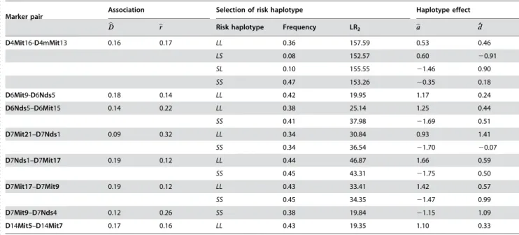
By assuming all the four haplotypes as a risk haplotype, respectively, the above model allows for the estimates of haplotype frequencies by the EM iteration at the higher hierarchy and of composite genotypic values by the EM iteration at the lower hierarchy. The estimated haplotype frequencies are used to estimate linkage disequilibrium based on equation (14) and the recombination fraction (r) based on equation (4). This estimation process is moved from the first (M1–M2) to last pair of markers (M6–M7) on chromosome 1 and then from chromosome 1 to 19. Table 3 tabulates the results of the MLEs of haplotype frequencies and log-likelihoods under the assumptions of different risk haplotypes. A total of 96 markers are sparsely located on 19 mouse chromosomes, with the estimated recombination fractions from the linkage disequilibrium model [8] consistent with those obtained from the linkage model [21]. Significant likelihood ratios for testing haplotype effects were determined by critical values obtained from the x2

-square distribution with two degrees of freedom with a Bonferroni adjustment to the type I error. The adjusted critical values for the two- and three-marker QTN models are 18.20 and 18.76, respectively, at the 5% significance level. Significant haplotype effects are detected for a total of eight marker pairs (Table 3), which include one pair on chromosome 4, two consecutive pairs on chromosome 6, four consecutive pairs on chromosome 7 and one pair on chromosome 14. For some pairs, multiple significant risk haplotypes were detected. Risk haplotypes purely composed of alleles inherited from the LG/J or SM/J parent exert a positive or negative additive effect on body weight, respectively. Based on the relative values of estimated additive and dominant effects, the significant marker pairs detected display partial dominant effects (Table 3).

The results from the three-marker model are basically consistent with those from the two-marker model (Table 4). The advantage of the three-marker model is that it incorporates the interferences between adjacent marker intervals into the estimation process and, thus, can potentially increase the estimation precision of haplotype effects.

DISCUSSION

Quantitative trait locus (QTL) mapping aims to identify narrow chromosomal segments for a quantitative trait by using a statistical method, and has proven its value to study the genetic architecture of the trait in a variety of species [6–8]. The limitations of this technique lie in its inability to characterize the structure and organization of DNA sequences and statistical difficulty in deriving the distribution of test statistics under the null hypothesis of no QTL [22]. At least partly for these reasons, despite thousands of QTL reported for different traits and populations, a very small portion of them have been cloned [9]. With the completion of the genome projects for several important organisms, a new line of thought in the post genomic era has begun to emerge for the identification of specific combinations of nucleotides or haplotypes that contribute to a complex quantitative trait [13,23].

(9)

a trait in experimental crosses. We used the principle of linkage disequilibrium analysis to characterize the linkage among different markers that is usually described by the recombination fractions in a commonly used F2population, initiated with two inbred lines. We established an interchangeable relationship between the linkage and linkage disequilibrium. The merit of this relationship in trait haplotyping includes the incorporation of interferences

between adjacent marker intervals into the estimation and test of haplotype effects when multiple markers are modelled simulta-neously.

The haplotyping model developed in this article was used to analyze a published F2 population of mouse [21], but we used microsatellite markers as the surrogate of SNPs so that we can detect the effects of haplotypes constructed by microsatellite

Table 3.The MLEs of haplotype frequencies and significant log-likelihood ratios (LR) by assuming different risk haplotypes in the F2

population of mice.

. . . .

Marker pair Association Selection of risk haplotype Haplotype effect

b D

D brr Risk haplotype Frequency LR2 baa dd^

D4Mit16-D4mMit13 0.16 0.17 LL 0.36 157.59 0.53 0.46

LS 0.08 152.57 0.60 20.91

SL 0.10 155.55 21.46 0.90

SS 0.47 153.26 20.35 0.18

D6Mit9-D6Nds5 0.18 0.14 LL 0.42 19.95 1.17 0.24

D6Nds5–D6Mit15 0.14 0.22 LL 0.38 25.14 1.25 0.44

SS 0.41 37.98 21.69 0.51

D7Mit21–D7Nds1 0.09 0.32 LL 0.34 30.84 0.93 1.41

SS 0.34 36.54 21.70 20.07

D7Nds1–D7Mit17 0.19 0.12 LL 0.44 46.87 1.66 0.59

SS 0.45 43.31 21.75 0.50

D7Mit17–D7Mit9 0.19 0.12 LL 0.43 33.41 1.42 0.57

SS 0.45 34.35 21.47 0.99

D7Mit9–D7Nds4 0.12 0.26 SS 0.38 19.84 21.15 1.09

D14Mit5–D14Mit7 0.17 0.16 LL 0.43 19.35 1.10 0.33

The results were obtained by using a two-SNP QTN model. doi:10.1371/journal.pone.0000732.t003

...

....

...

....

...

....

...

....

...

....

...

....

...

....

...

....

...

Table 4.The MLEs of haplotype frequencies and significant log-likelihood ratios (LR) by assuming different risk haplotypes in the F2

population of mice.

. . . .

Marker pair Selection of risk haplotype Haplotype effect

Risk haplotype Frequency LR2 ^aa ^dd

D4Mit45–D4Mit16–D4Mit13 LLL 0.29 124.70 0.40 0.61

LLS 0.07 121.34 1.08 21.00

LSL 0.01 122.58 21.88 22.56

LSS 0.07 122.08 20.44 1.40

SLL 0.07 122.14 0.80 0.12

SLS 0.01 132.86 -

-SSL 0.09 122.33 21.32 1.09

SSS 0.40 123.65 20.55 0.28

D6Mit9–D6Nds5–D6Mit15 SSS 0.34 22.65 21.51 0.39

D7Mit21–D7Nds1–D7Mit17 LLL 0.29 38.28 0.81 1.85

SSS 0.30 33.74 21.80 0.09

D7Nds1–D7Mit17–D7Mit9 LLL 0.38 34.39 1.48 0.47

SSS 0.40 32.18 21.61 0.61

D7Mit17–D7Mit9–D7Nds4 LLL 0.33 21.74 1.20 0.45

SSS 0.33 29.41 21.60 1.36

D14Nds1–D14Mit5–D14Mit7 LLL 0.30 19.55 1.44 20.50

The results were obtained by using a three-SNP QTN model. doi:10.1371/journal.pone.0000732.t004

....

...

....

...

....

...

....

...

....

...

....

...

....

...

....

...

....

...

(10)

alleles. The whole-genome of mouse was scanned for haplotype effects on body weight by a two- and multi-marker model, respectively. Consistent results were observed from the two models, which suggests that four regions in mouse chromosomes 4, 6, 7, and 14 contribute to variation in body weight. These findings are in a good agreement with those from traditional interval QTL mapping [21]. But our haplotype discovery is more informative in terms of the characterization of specific haplotype structure and organization responsible for trait variation.

We have proposed a new model for haplotyping a quantitative trait in the F2progeny population. The tenet of the model can be extended to haplotype a complicated trans-generational pedigree, founded with multiple original parents and involving individuals with different relatedness. The model can also be modified to dissect the epistatic effects of different genes [23] and the interaction of genes with environment. For these extensions, haplotype selection aimed to detect the risk haplotypes that are expressed differently from the others present many challenges, but

is crucial for the facilitation of the process of detecting the association between haplotype diversity and phenotypic variation. Our haplotyping model offers a powerful tool for positional cloning of QTL that are important for a complex trait. Flint et al. [9] reviewed the potential of currently available cloning strategies, such as probabilistic ancestral haplotype reconstruction, Yin-Yang crosses and in silico analysis of sequence variants, to identify genes that underlie QTL in rodents. Our model, in conjunction with these strategies, may open a new gateway for the illustration of a detailed picture of the genetic architecture for a complex trait.

ACKNOWLEDGMENTS

Author Contributions

Conceived and designed the experiments: RW. Performed the experi-ments: JC. Analyzed the data: WH SW TL. Wrote the paper: RW.

REFERENCES

1. Lander ES, Botstein D (1989) Mapping Mendelian factors underlying quantitative traits using RFLP linkage maps. Genetics 121: 185–199. 2. Lynch M, Walsh B (1998) Genetics and Analysis of Quantitative Traits. Sinauer

Associates, Sunderland, MA.

3. Jansen RC, Stam P (1994) High resolution mapping of quantitative traits into multiple loci via interval mapping. Genetics 136: 1447–1455.

4. Zeng Z-B (1994) Precision mapping of quantitative trait loci. Genetics 136: 1457–1468.

5. Kao C-H, Zeng Z-B, Teasdale RD (1999) Multiple interval mapping for quantitative trait loci. Genetics 152: 1203–1216.

6. Mackay TFC (2001) Quantitative trait loci inDrosophila. Nat Rev Genet 2: 11–20.

7. Frary A, Nesbitt TC, Frary A, Grandillo S, van der Knaap E, et al. (2000)fw2.2: A quantitative trait locus key to the evolution of tomato fruit size. Science 289: 85–88.

8. Li CB, Zhou AL, Sang T (2006) Rice domestication by reducing shattering. Science 311: 1936–1939.

9. Flint J, Valdar W, Shifman S, Mott R (2005) Strategies for mapping and cloning quantitative trait genes in rodents. Nat Rev Genet 6: 271–286.

10. Churchill GA, Doerge RW (1994) Empirical threshold values for quantitative trait mapping. Genetics 138: 963–971.

11. Judson R, Stephens JC, Windemuth A (2000) The predictive power of haplotypes in clinical response. Pharmacogenomics 1: 15–26.

12. Bader JS (2001) The relative power of SNPs and haplotype as genetic markers for association tests. Pharmacogenomics 2: 11–24.

13. Liu T, Johnson JA, Casella G, Wu RL (2004) Sequencing complex diseases with HapMap. Genetics 168: 503–511.

14. Lou X-Y, Casella G, Littell RC, Yang MKC, Wu RL (2003) A haplotype-based algorithm for multilocus linkage disequilibrium mapping of quantitative trait loci with epistasis in natural populations. Genetics 163: 1533–1548.

15. Patil N, Berno AJ, Hinds DA, Barrett WA, Doshi JM, et al. (2001) Blocks of limited haplotype diversity revealed by high-resolution scanning of human chromosome 21. Science 294: 1719–1723.

16. Zhang K, Deng M, Chen T, Waterman MS, Sun F (2002) A dynamic programming algorithm for haplotype block partitioning. Proc Natl Acad Sci 99: 7335–7339.

17. Sebastiani P, Lazarus SW, Kunkel LM, Kohane IS, Ramoni M (2003) Minimal haplotype tagging. Proc Natl Acad Sci 100: 9900–9905.

18. Eyheramendy S, Marchini J, McVean G, Myers S, Donnelly P (2007) A model-based approach to capture genetic variation for future association studies. Genome Res 17: 88–95.

19. Louis TA (1982) Finding the observed information matrix when using the EM algorithm. J Roy Stat Soc Ser B 44: 226–233.

20. Burnham KP, Andersson DR (1998) Model Selection and Inference. A Practical Information-Theoretic Approach. Springer: New York.

21. Vaughn TT, Pletscher LS, Peripato A, King-Ellison K, Adams E, et al. (1999) Mapping quantitative trait loci for murine growth - A closer look at genetic architecture. Genet Res 74: 313–322.

22. Lander ES, Schork NJ (1994) Genetic dissection of complex traits. Science 265: 2037–2048.