www.clim-past.net/7/473/2011/ doi:10.5194/cp-7-473-2011
© Author(s) 2011. CC Attribution 3.0 License.
of the Past
Abrupt rise in atmospheric CO
2
at the onset of the Bølling/Allerød:
in-situ ice core data versus true atmospheric signals
P. K¨ohler1, G. Knorr1,2, D. Buiron3, A. Lourantou3,*, and J. Chappellaz3
1Alfred Wegener Institute for Polar and Marine Research (AWI), P.O. Box 120161, 27515 Bremerhaven, Germany 2School of Earth and Ocean Sciences, Cardiff University, Cardiff, Wales, UK
3Laboratoire de Glaciologie et G´eophysique de l’Environnement, (LGGE, CNRS, Universit´e Joseph Fourier-Grenoble),
54b rue Moli`ere, Domaine Universitaire BP 96, 38402 St. Martin d’H`eres, France
*now at: Laboratoire d’Oc´eanographie et du Climat (LOCEAN), Institut Pierre Simon Laplace, Universit´e P. et M. Curie
(UPMC), Paris, France
Received: 24 June 2010 – Published in Clim. Past Discuss.: 11 August 2010 Revised: 15 March 2011 – Accepted: 24 March 2011 – Published: 4 May 2011
Abstract. During the last glacial/interglacial transition the Earth’s climate underwent abrupt changes around 14.6 kyr ago. Temperature proxies from ice cores revealed the onset of the Bølling/Allerød (B/A) warm period in the north and the start of the Antarctic Cold Reversal in the south. Further-more, the B/A was accompanied by a rapid sea level rise of about 20 m during meltwater pulse (MWP) 1A, whose exact timing is a matter of current debate. In-situ measured CO2in
the EPICA Dome C (EDC) ice core also revealed a remark-able jump of 10±1 ppmv in 230 yr at the same time. Allow-ing for the modelled age distribution of CO2in firn, we show
that atmospheric CO2could have jumped by 20–35 ppmv in
less than 200 yr, which is a factor of 2–3.5 greater than the CO2signal recorded in-situ in EDC. This rate of change in
at-mospheric CO2corresponds to 29–50% of the anthropogenic
signal during the last 50 yr and is connected with a radiative forcing of 0.59–0.75 W m−2. Using a model-based airborne
fraction of 0.17 of atmospheric CO2, we infer that 125 Pg
of carbon need to be released into the atmosphere to pro-duce such a peak. If the abrupt rise in CO2at the onset of
the B/A is unique with respect to other Dansgaard/Oeschger (D/O) events of the last 60 kyr (which seems plausible if not unequivocal based on current observations), then the mecha-nism responsible for it may also have been unique. Available δ13CO2 data are neutral, whether the source of the carbon
is of marine or terrestrial origin. We therefore hypothesise that most of the carbon might have been activated as a
conse-Correspondence to:P. K¨ohler (peter.koehler@awi.de)
quence of continental shelf flooding during MWP-1A. This potential impact of rapid sea level rise on atmospheric CO2
might define the point of no return during the last deglacia-tion.
1 Introduction
Measurements of CO2 over Termination I (20–10 kyr BP)
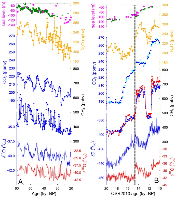
from the EPICA Dome C (EDC) ice core (Monnin et al., 2001; Lourantou et al., 2010) (Fig. 1b) are temporally higher resolved and more precise than CO2records from other ice
cores (Smith et al., 1999; Ahn et al., 2004). They have an uncertainty (1σ ) of 1 ppmv or less (Monnin et al., 2001; Lourantou et al., 2010). In these in-situ measured data in EDC, CO2abruptly rose by 10±1 ppmv between 14.74 and
14.51 kyr BP on the most recent ice core age scale (Lemieux-Dudon et al., 2010). This abrupt CO2rise is therefore
syn-chronous with the onset of the Bølling/Allerød (B/A) warm period in the North (Steffensen et al., 2008), the start of the Antarctic Cold Reversal in the South (Stenni et al., 2001), as well as abrupt rises in the two other greenhouse gases CH4
(Spahni et al., 2005) and N2O (Schilt et al., 2010).
Further-more, the B/A is accompanied by a rapid sea level rise of about 20 m during meltwater pulse (MWP) 1A (Peltier and Fairbanks, 2007), whose exact timing is matter of current de-bate (e.g. Hanebuth et al., 2000; Kienast et al., 2003; Stanford et al., 2006; Deschamps et al., 2009).
-140 -120 -100 -80 -60 -140 -120 -100 -80 -60
sea
le
v
e
l
(m
)
180 200 220 240 260 280 300N
2O
(pp
b
v)
190 200 210 220 230 240 250 260 270 190 200 210 220 230 240 250 260 270C
O
2(p
p
mv)
300 400 500 600 700 800C
H
4(pp
b
v)
-42.5 -40.0 -37.5 -35.0 1 8O
(
o
/
oo
)
60 50 40 30 20
Age (kyr BP)
-42.5 -40.0 -37.5 -35.0 -32.5 1 8
O
(
o/
o o)
A
-140 -120 -100 -80 -60 -140 -120 -100 -80 -60sea
le
v
el
(m
)
180 200 220 240 260 280 300N
2O
(ppb
v)
190 200 210 220 230 240 250 260 270 190 200 210 220 230 240 250 260 270C
O
2(p
pmv)
300 400 500 600 700 800C
H
4(ppb
v)
-45 -42 -39 -36 -33 -30 1 8O
(
o
/
oo
)
-460 -440 -420 -400 -380D
(
o
/
oo
)
20 18 16 14 12 10
QSR2010 age (kyr BP)
B
0 500 1000 1500 2000 Time since last exchange with atmosphere (yr)
0 1 2 3 4 5 6
Probability
(
o /oo
)
EPRE=213yr
EB/A=400yr
ELGM=590yr
LGM CO2firn model
LGM lognormal B/A lognormal
PRE CO2firn model
PRE lognormal
Fig. 2.Age distribution PDF of CO2as a function of climate state, here pre-industrial (PRE), Bølling/Allerød (B/A) and LGM condi-tions. Calculation with a firn densification model (Joos and Spahni, 2008) (solid lines, for PRE and LGM) and approximations of all three climate states by a log-normal function (broken lines). For all functions the expected mean values, or widthE, are also given.
accumulation rate because of the movement of gases in the firn above the close-off depth and before its enclosure in gas bubbles in the ice. To infer the transfer signature of the true atmospheric CO2signal out of in-situ ice core CO2
measure-ments, the latter has to be deconvoluted with the ice-core-specific age distribution probability density function (PDF). Based on a firn densification model (Joos and Spahni, 2008), this age distribution PDF describing the elapsed time since the last exchange of the CO2molecules with the atmosphere
(Fig. 2) reveals for EDC a width of approximately 200 and 600 yr for climate conditions of pre-industrial times (PRE) and the Last Glacial Maximum (LGM), respectively. These wide age distributions implicate that the CO2measured
in-situ, especially in ice cores with low accumulation rates (such as EDC), differs from the true atmospheric signal when CO2
changes abruptly.
In the following we will deconvolve the atmospheric CO2
signal connected with this abrupt rise in CO2measured
in-situ in the EDC ice core, allowing for the age distribution PDF during the onset of the B/A. We furthermore use sim-ulations of a global carbon cycle box model to develop and test a hypotheses which might explain the abrupt rise in at-mospheric CO2.
2 Methods
2.1 Age distribution PDF of CO2
The age distributions PDF of CO2or CH4 are functions of
the climate state and the local site conditions of the ice core.
In Fig. 2, the age distributions PDF of CO2in the EDC ice
core for pre-industrial (PRE) and LGM conditions based on calculations with a firn densification model (Joos and Spahni, 2008) are shown. The resulting age distribution PDF for CO2
can be approximated with reasonable accuracy (r2=90– 94%) by a log-normal function (K¨ohler et al., 2010b):
y= 1
x·σ·√2π·e
−0.5ln(x)σ−µ2
(1) withx (yr) as the time elapsed since the last exchange with the atmosphere. This equation has two free parametersµand σ. For simplcity, we have chosenσ=1, which leads to an expected value (mean) Eof the PDF of
E=eµ+0.5. (2)
Theexpected value Eis described aswidthof the PDF in the terminology of gas physics, a terminology which we will also use in the following.Eshould not be confused with the most likely valuedefined by the location of the maximum of the PDF.
Our choice to use a log-normal function (Eq. 1) for the age distribution PDF was motivated by the good represen-tation of firn densification model output (r2≥90%) and its dependency on only one free parameter, which can be ob-tained from models. Other approaches using, for example, a Green’s function are also possible (see Trudinger et al., 2002, and references therein).
In the case of the CO2jump at 14.6 kyr BP, one has to
con-sider that the atmospheric records are much younger than the surrounding ice matrix; indeed, the CO2jump is embedded
between 473 and 480 m in glacial ice (Monnin et al., 2001; Lourantou et al., 2010) with low temperatures and low accu-mulation rates. However, from a model of firn densification which includes heat diffusion, it is known that the close-off of the gas bubbles in the ice matrix is not a simple func-tion of the temperature of the surrounding ice (Goujon et al., 2003). Heat from the surface diffuses down to the close-off region in a few centuries, depending on site-specific condi-tions. This implies that atmospheric gases during the onset of the B/A were not trapped by conditions of either the LGM or the Antarctic Cold Reversal, but by some intermediate state. New calculations with this firn densification model (Goujon et al., 2003) give a width of the age distribution PDFEB/A
of about 400 yr with a relative uncertainty (1σ) of 14% at the onset of the B/A (Fig. 3). The widthEitself varies during the jump into the B/A between 380 and 420 yr; we therefore conservatively estimateEB/A to lie between 320 to 480 yr
with our best-guess estimate ofEB/A=400 yr in-between.
The performance of the applied gas age distribution PDF (Eq. 1) is tested with ice core CH4data for the time window
190
200
210
220
230
240
250
260
270
280
290
CO
2
(ppmv)
700
600
500
400
300
200
100
0
width
E
of
age
distribution
(yr)
20 18 16 14 12 10 8 6 4 2 0
QSR2010 age (kyr BP)
-440
-420
-400
-380
-360
D
(
o
/
oo)
Fig. 3.Evolution of the widthEof the age distribution PDF (±1σ) during the last 20 kyr (red squares) calculated with a firn densifi-cation model including heat diffusion (Goujon et al., 2003). Green diamonds represent the results for the LGM and pre-industrial cli-mate with another firn densification model (Joos and Spahni, 2008). Please note reverse y-axis. Top: EDC CO2(Monnin et al., 2001; Lourantou et al., 2010). Bottom: EDCδD data (Stenni et al., 2001). All records are on the new age scale QSR2010 (Lemieux-Dudon et al., 2010).
therefore justified to apply Eq. (1) to convolve the CO2signal
which might be recorded in the EDC ice core. 2.2 Carbon cycle modelling
In order to determine how fast carbon injected into the atmo-sphere is taken up by the ocean, we used the carbon cycle box model BICYCLE (K¨ohler and Fischer, 2004; K¨ohler et al., 2005a, 2010b). The model version used here and its forcing over Termination I are described in detail in Lourantou et al.
(2010). Furthermore, we tried to determine of which origin (terrestrial or marine) the carbon might have been by com-paring the simulated and measured atmosphericδ13CO2
fin-gerprint during the carbon release event. Similar approaches (identifying processes based on theirδ13C signature) were applied earlier for the discussion of the atmosphericδ13CO2
record over the whole Termination I (Lourantou et al., 2010) and longer timescales (K¨ohler et al., 2010b). Here, we re-strict the analysis to the question of whether the observed signal might be generated by terrestrial or marine processes only.
Briefly, BICYCLE consists of modules of the ocean (10 boxes distinguishing surface, intermediate and deep ocean in the Atlantic, Southern Ocean and Indo-Pacific), a glob-ally averaged terrestrial biosphere (7 boxes), a homoge-neously mixed one-box atmosphere, and a relaxation ap-proach to account for carbonate compensation in the deep ocean (sediment-ocean interaction). The model calculates the temporal development of its prognostic variables over time as functions of changing boundary conditions, repre-senting the climate forcing. These prognostic variables are (a) carbon (as dissolved inorganic carbon DIC in the ocean), (b) the carbon isotopesδ13C,114C, and (c) additionally in the ocean total alkalinity, oxygen and phosphate. The terres-trial module accounts for different photosynthetic pathways (C3or C4), which is relevant for the temporal development
of the13C cycle.
Here, the model is equilibrated for 4000 yr for climate conditions typical before the onset of the B/A. The At-lantic meridional overturning circulation (AMOC) is in an off mode. Simulations with the AMOC in an on mode lead to a different background state of the carbon cycle (atmo-sphericpCO2is then 255 ppmv versus 223 ppmv in the off
mode), but the amplitudes in the atmospheric CO2rise
dif-fer by less than 3 ppmv between both settings. Scenarios in which the AMOC amplifies precisely at the onset of the B/A warm period are not explicitly considered here, but are im-plicitly covered in the marine scenario. An amplification of the AMOC would lead to stadial/interstadial variations typ-ical for the bipolar seesaw. Such behaviour was found for the onset of other D/O events in MIS 3 (Barker et al., 2010) during which CO2started to fall and not to rise as observed
for the B/A. Based on this analogy, our working hypothe-sis is that the main processes connected with changes in the AMOC play a minor role for the abrupt rise in atmospheric CO2around 14.6 kyr BP (see Sect. 3.2 for details).
The simulated jump of CO2 is generated by the
atmosphere. Our best guess injection amplitude of 125 PgC corresponds to constant injection fluxes of 2.5 Pg C yr−1(in
50 yr) to 0.42 Pg C yr−1(in 300 yr) over the whole release
pe-riod. The fastest injection (in 50 yr) with the largest annual flux has been motivated by the abruptness in the climate sig-nals recorded in the NGRIP ice core (Steffensen et al., 2008). It is furthermore assumed that the injected carbon is either of terrestrial or marine origin. These two scenarios differ only in their carbon isotopic signature:
Terrestrial scenario:theδ13C signature is based on a study with a global dynamical vegetation model (Scholze et al., 2003), which calculates a mean global isotopic fractionation of the terrestrial biosphere of 17.7‰ for the present day. We have to consider a larger fraction of C4plants during colder
climates and lower atmosphericpCO2(Collatz et al., 1998),
as found at the onset of the B/A. This implies that about 20 and 30% of the terrestrial carbon is of C4origin for present
day and LGM, respectively (K¨ohler and Fischer, 2004). The significantly smaller isotopic fractionation during C4
photo-synthesis (about 5‰) in comparison to C3 photosynthesis
(about 20‰) (Lloyd and Farquhar, 1994) therefore reduces the global mean terrestrial fractionation to 16‰. With an at-mosphericδ13CO2signature of about−6.5‰, the terrestrial
biosphere has a meanδ13C signature of−22.5‰.
Marine scenario:in this scenario we assume that old car-bon from the deep ocean heavily depleted in δ13C might upwell and outgas into the atmosphere. Today’s values of oceanicδ13C in the deep Pacific are about 0.0‰ (Kroopnick, 1985). From reconstructions (Oliver et al., 2010), it is known that during the LGM deep oceanδ13C was on average about 0.5‰ smaller, thusδ13CLGM=−0.5‰. During out-gassing,
mainly in high latitudes, we consider a net isotopic fraction-ation of 8‰ (Siegenthaler and M¨unnich, 1981). This would lead toδ13C=−8.5‰ in the carbon injected into the atmo-sphere if it were of marine origin.
The signals of simulated atmospheric CO2 and δ13CO2
plotted in the figures are derived by subtracting simulated CO2andδ13CO2of a reference run without carbon injections
from our scenarios. The anomalies1(CO2) and1(δ13CO2)
are then added to the starting point of the CO2jump (δ13CO2
drop) into the B/A, which we define as 228 ppmv (−6.76‰) at 14.8 kyr BP. In doing so, existing equilibration trends (which will exist even for longer equilibration periods due to the sediment-ocean interaction) are eliminated. The simu-lated atmospheric CO2(δ13CO2) at the end of the
equilibra-tion period was 223 ppmv (−6.54‰). Our modelling exer-cise is therefore only valid for an interpretation of the abrupt CO2 rise of 10 ppmv in the in-situ data of EDC. The
mis-match in CO2 and δ13CO2 between simulations and EDC
data before 15 kyr BP and after 14.2 kyr BP, is therefore ex-pected (Figs. 4b, 4d, 5b, 5d, 7).
3 Results and discussions
3.1 Assessing the size of the carbon injection
We first estimate roughly the amount of carbon necessary to be injected as CO2 into the atmosphere to produce a
long-term jump of 10 ppmv using the airborne fraction f. The long-term (centuries to millennia) airborne fractionf of CO2
can be approximated from the buffer or Revelle factor (RF) of the ocean on atmospheric pCO2 rise. The present day
mean surface ocean Revelle factor (Sabine et al., 2004a) is about 10. With
RF=1pCO2/pCO2
1DIC/DIC (3)
and the content of C at the beginning of the B/A in the atmosphere (CA=500 Pg C≈235 ppmv) and in the ocean
(CO=37 500 Pg C=75· CA) it is
f= 1pCO2 1pCO2+1DIC=
1
1+RF75 =0.118. (4) Thus, the lower end of the range of the airborne fractionf is about 0.12 (given by Eq. 4), while the upper end of the range might be derived from modern anthropogenic fossil fuel emissions to about 0.45 (Le Qu´er´e et al., 2009). Please note thatf estimated with Eq. (4) assumes a passive (con-stant) terrestrial biosphere, while in the estimate off from fossil fuel emissions (Le Qu´er´e et al., 2009), the terrestrial carbon cycle is assumed to take up about a third of the an-thropogenic C emissions. We take the range off between 0.12 and 0.45 as a first order approximation and assumef during the B/A to lie in-between. This implies that a long-term rise in atmospheric CO2of 10 ppmv (equivalent to a rise
in the atmospheric C reservoir by 21.2 Pg C) can be generated by the injection of 47 to 180 Pg C into the atmosphere.
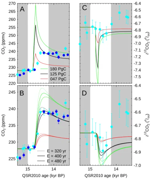
We further refine this amplitude to 125 Pg C (equivalent to f=0.17) by using the global carbon cycle box model BICY-CLE. The model then generates atmospheric CO2 peaks of
20–35 ppmv, depending on the abruptness of the C injection (Fig. 4a). All scenarios with release times of 50–200 yr fulfil the EDC ice core data requirements after the application of the age distribution PDF (Fig. 4b). The acceptable scenarios imply rates of change in atmospheric CO2of 13–70 ppmv per
century, a factor of 3–16 higher than in the EDC data. Our fastest scenario (release time of 50 yr) has a rate of change in atmospheric CO2, which is still a factor of two smaller than
the anthropogenic CO2rise of 70 ppmv during the last 50 yr
(Keeling et al., 2009). For comparison, in the less precise CO2data points taken from the Taylor Dome (Smith et al.,
1999) and Siple Dome (Ahn et al., 2004) ice cores, the abrupt rise in CO2at the onset of the B/A is recorded with 15±2 and
19±4 ppmv, respectively (Fig. 4a), with changing rates in ice core CO2of∼4–6 ppmv per century. This already indicates
that at 14.6 kyr BP, CO2 measured in-situ in EDC differed
220 225 230 235 240 245 250 255 260 265 270
CO
2
(ppmv)
SD (Ahn 2004) TD (Smith 1999) EDC (Lourantou 2010) EDC (Monnin 2001)
A
220 225 230 235 240 245 250 255 260 265 270
CO
2
(ppmv)
15 14
SD age (kyr BP)
15 14
QSR2010 and TD age (kyr BP) 225
230 235 240 245
CO
2
(ppmv)
B
-7.5 -7.4 -7.3 -7.2 -7.1 -7.0 -6.9 -6.8 -6.7 -6.6 -6.5 -6.4
1
3 CO
2
(
o /oo
)
M 050 yr T 300 yr T 250 yr T 200 yr T 150 yr T 100 yr T 050 yr
C
15 14
QSR2010 age (kyr BP) -7.0 -6.9 -6.8 -6.7 -6.6 -6.5 -6.4
1
3 CO
2
(
o /oo
)
D
Fig. 4.Simulations with the carbon cycle box model BICYCLE for an injection of 125 Pg C into the atmosphere. Injected carbon was either of terrestrial (T:δ13C=−22.5‰) or marine (M:δ13C=−8.5‰) origin. Release of terrestrial C occurred between 50 and 300 yr. Marine C was released in 50 yr (grey), but is identical to the terrestrial release in A, B.(A)Atmospheric CO2from simulations and from EDC (Monnin et al., 2001; Lourantou et al., 2010) on the new age scale QSR2010 (Lemieux-Dudon et al., 2010), Siple Dome (Ahn et al., 2004) (SD, on its own age scale on top x-axis) and Taylor Dome (Smith et al., 1999) (TD, on revised age scale as in Ahn et al., 2004). All CO2data has been synchronised to the CO2jump. (B)Simulated CO2values potentially be recorded in EDC and EDC data. The simulated values are derived by the application of the gas age distribution PDF of the hypothetical atmospheric CO2values plotted in (A), followed by a shift in the age scale by the widthEB/A=400 yr towards younger ages. (C, D)The same simulations for atmosphericδ13CO2, cyan dots are new EDCδ13CO2data (Lourantou et al., 2010). Only the dynamics between 15.0 and 14.2 kyr BP (white band) are of interest here and should be compared to the ice core data.
The uncertainty in the size of the CO2peak given by the
variability in the width EB/A of the age distribution PDF
and by the range in the airborne fractionf lead to slightly different results. The differences inEB/A between 320 and
480 yr give forf=0.17 variations in the atmospheric CO2
peak height of less than 1 ppmv from the standard case and these results are still within uncertainties of the ice core data (Fig. 5b). We show in Fig. 5a and 5c how the atmospheric
CO2andδ13CO2would look like for the upper (f=0.45)
and lower (f =0.12) end-of-range values in the airborne fractionf, if simulated with our carbon cycle box model us-ing a release time of 100 yr. The signal potentially recorded in EDC is achieved after applying the age distribution PDF (Fig. 5b, 5d). Atmospheric CO2 rose by 10 ppmv only in
in the atmosphere would be 42 ppmv, which is 13 ppmv larger than the 29 ppmv in our reference case, leading to a long-term CO2 jump of 16 ppmv in a hypothetical EDC
ice core. After the application of the age distribution PDF, both extreme cases forf were not in line with the evidence from the ice core data.
3.2 Fingerprint analysis and process detection – the shelf flooding hypothesis
But what generated this jump of CO2 at the onset of the
B/A? Changes in the near-surface temperature and in the AMOC had massive impacts on the reorganisation of the ter-restrial and the marine carbon cycle (K¨ohler et al., 2005b; Schmittner and Galbraith, 2008), respectively. This led to CO2 amplitudes of about 20 ppmv during D/O events
(Ahn and Brook, 2008). At the onset of the B/A the tem-perature changes in the northern and southern high lati-tudes as recorded in Greenland and in the central Antarctic plateau followed the typical pattern of the bipolar seesaw that also characterised the last glacial cycle (EPICA-community-members, 2006; Barker et al., 2009): gradual warming in the South during a stadial cold phase in the North switched to gradual cooling at the onset of a abrupt temperature rise in the North (Fig. 1a). These interhemispheric patterns were identified for all D/O events during Marine Isotope Stage 3 (MIS 3) and for the B/A as D/O event 1 (EPICA-community-members, 2006) (Fig. 1). In contrast to all D/O events dur-ing MIS 3, in which CO2 started to decline at the onset of
Greenland warming (Ahn and Brook, 2008), CO2abruptly
increased around 14.6 kyr BP. This temporal pattern strongly suggests that changes in the AMOC are not the main source of the detected CO2jump at the onset of the B/A, since the
general trend of the CO2evolution during the D/O events in
MIS 3 is, based on existing data, of opposite sign.
However, we have to acknowledge that the mean temporal resolution1t of CO2 data obtained from various other ice
cores in MIS 3 is with1t=150–1000 yr much larger than for the CO2record of EDC during Termination I (1t=92 yr,
Table 1). For this comparison, one needs to consider that those data with the highest temporal resolution (Byrd,1t= 150 yr, Neftel et al., 1988) are those with the highest mea-surement uncertainty (mean 1σ =4 ppmv, for comparison EDC: mean 1σ≤1 ppmv). All other CO2ice core records in
MIS 3 have1t >500 yr. Furthermore, present day accumu-lation rates in these other ice cores are 2–5 times higher than in EDC, implying an approximately 2–5 times lower mean widthEof the gas age distribution PDF in the other ice cores (Spahni et al., 2003) and thus a smaller smoothing effect of the gas enclosure (Table 1). Therefore, the possibility that similar abrupt CO2rises in the true atmospheric signal also
exist during other D/O events can not be excluded, although the data evidence from the overlapping CO2records of the
Taylor Dome and Byrd ice cores does not seem to allow such dynamics for the time between 20–47 kyr BP (Table 1, Ahn
and Brook, 2007). Furthermore, the rate of change in CO2at
the onset of the B/A is not unique for the last glacial cycle. In the time window 65–90 kyr, BP (belonging to MIS 4 and 5) CO2measured in-situ in the Byrd ice core (Ahn and Brook,
2008) rose several times abruptly by up to 22±4 ppmv in 200 yr, sometimes synchronous with northern warming (sim-ilar as for the B/A), and sometimes not. It needs to be tested if a similar mechanism as proposed here was also responsible for these CO2jumps. An ice core with higher resolution,
e.g. the West Antarctic Ice Sheet (WAIS) Divide Ice Core, might help to clarify the magnitude and shape of the abrupt rise in atmospheric CO2during the onset of the B/A and its
uniqueness with respect to other D/O events in MIS 3. The WAIS Divide Ice Core exhibits a present day accumulation rate of 24 g cm−2yr−1(Morse et al., 2002), which is nearly
an order of magnitude larger than EDC and 50% larger than Byrd (Table 1).
Our working hypothesis also implies that the changes in the AMOC connected with the bipolar seesaw pattern ob-served for B/A and other D/O events during MIS 3 were similar. Proxy-based evidence supports this assumed simi-larity: A reduction of the AMOC to a similar strength dur-ing various stadials (Younger Dryas, Heinrich Stadials 1 and 2) was deduced from 231Pa/230Th (McManus et al., 2004; Lippold et al., 2009). These results were also supported by reconstructed ventilation ages in the South Atlantic off the coast of Brazil (Mangini et al., 2010). The magnitude of the AMOC amplification during a stadial/interstadial transition is more difficult to deduce from proxy data. However, Barker et al. (2010) recently reconstructed ventilation changes in the South Atlantic Ocean and found a deep expansion of the North Atlantic Deep Water export during the B/A (following Heinrich Stadial 1), similar to results during the D/O event 8 around 38 kyr BP (following Heinrich Stadial 4). Taken to-gether the data-based evidence indicates that (a) the AMOC was shut down in a very similar way during Heinrich Sta-dials, and (b) the magnitude and the characteristics of the AMOC amplification at the B/A was not exceptional (Knorr and Lohmann, 2007; Barker et al., 2010). Thus, the AMOC amplification during the B/A seemed to be similar to some D/O events in MIS 3 following Heinrich Stadials. Both in-dications support our assumption that changes in the AMOC can not explain the majority of the abrupt rise in atmospheric CO2at the onset of the B/A. The robustness of our
hypoth-esis with respect to the uniqueness of the event might also be tested by future higher resolved CO2data, as mentioned
above.
To constrain the origin of the released carbon further, we investigate the two hypotheses, that the carbon was only of either terrestrial or marine origin. Our two scenarios vary only in the isotopic signature of the injected C (terrestrial: δ13CO2=−22.5‰, marine: δ13CO2=−8.5‰). We compare
220 225 230 235 240 245 250 255 260 265 270
CO
2
(ppmv)
047 PgC 125 PgC 180 PgC
A
15 14
QSR2010 age (kyr BP) 225
230 235 240 245
CO
2
(ppmv)
E = 480 yr E = 400 yr E = 320 yr
B
-7.5 -7.4 -7.3 -7.2 -7.1 -7.0 -6.9 -6.8 -6.7 -6.6 -6.5 -6.4
1
3 CO
2
(
o /oo
)
C
15 14
QSR2010 age (kyr BP) -7.0 -6.9 -6.8 -6.7 -6.6 -6.5 -6.4
1
3 CO
2
(
o /oo
)
D
Fig. 5. Influence of (i) the amount of carbon injected in the atmosphere and of (ii) the details of the gas age distribution on both the atmospheric signal and that potentially recorded in EDC. The amount of carbon injected in the atmosphere(A, C)covers the range derived from an airborne fractionf between 12 and 45% from 47 to 180 Pg C with our reference scenario of 125 Pg C in bold. Injections occurred in 100 yr with terrestrialδ13C signature. In the filter function of the gas age distribution(B, D)the widthEvaries from 320 yr to 480 yr, our best-estimated gas age widthEat the onset of the B/A of 400 yr in the solid line, representing the range given by the firn densification model including heat diffusion (Goujon et al., 2003), as plotted in Fig. 3. Only the dynamics between 15.0 and 14.2 kyr BP (white band) are of interest here and should be compared with the ice core data.
small dip of−0.14±0.14‰ inδ13CO2measured in-situ in
EDC might be generated by terrestrial C released in less than three centuries (Fig. 4c, 4d). The marine scenario leads to changes inδ13CO2 of less than−0.03‰ (Fig. 4d). Within
the uncertainty in so-far-published ice coreδ13CO2of 0.10‰
(1σ), this marine scenario seems less likely than the terres-trial one, but it can not be excluded. All together, thisδ13CO2
fingerprint analysis shows that all terrestrial or marine sce-narios seemed to be possible, but a further constraint is, based on the given data so far, not possible. New measured, but up to now unpublishedδ13CO2 data does not seem to lead to
different conclusions (Fischer et al., 2010).
Table 1. Available high resolution ice core CO2records over the last glacial cycle in comparison to the EPICA Dome C data covering Termination I.
ice core time window # mean1t present day CO2 reference
acc. rate∗ mean 1σ
units kyr BP – yr g cm−2yr−1 ppmv
EPICA Dome C 10–20 109 92 3 ≤1 Monnin et al. (2001); Lourantou et al. (2010)
Taylor Dome 20–60 73 550 7 ≤1 Inderm¨uhle et al. (2000)
Siple Dome 20–41 21 1000 12 2 Ahn et al. (2004)
Byrd 30–47 113 150 16 4 Neftel et al. (1988) as published in Ahn and Brook (2007)
Byrd 47–65 34 530 16 2 Ahn and Brook (2007)
Byrd 65–91 76 342 16 2 Ahn and Brook (2008)
∗Taken from the compilation of Ahn et al. (2004).
varied depending on site location and reconstruction method. However, Sunda Shelf data (Hanebuth et al., 2000; Kienast et al., 2003) and recent evidence from Tahiti (Deschamps et al., 2009) point to a timing of MWP-1A at 14.6 kyr BP, in parallel to the temperature rise and the abrupt rise in CO2
at the onset of the B/A. Sea level records (Thompson and Goldstein, 2007) suggest that large shelf areas which were exposed around 30 kyr BP were re-flooded within centuries by MWP-1A. The terrestrial ecosystems had thus ample time to develop dense vegetation and accumulate huge amounts of carbon, which could thus be released abruptly. In contrast to MWP-1A, the gradual sea level rise during MIS 3 allowed for CO2equilibration between atmosphere and ocean. This
difference between the B/A and other D/O events in MIS 3 in both the rate of sea level rise and the return interval of shelf flooding events (used for terrestrial carbon build-up) suggests that other rapid CO2 jumps are probably not caused by the
process of shelf flooding.
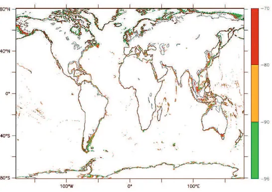
We estimate from bathymetry (Smith and Sandwell, 1997, version 12.1) that 2.2, 3.2 or 4.0×10¹²m2 of land were flooded during MWP-1A for sea level rising between−96 m and −70 m by 16, 20 or 26 m, respectively. This covers the different reconstructions published for MWP-1A (from
−96 m to−80 m, from−90 m to−70 m, or a combination of both, Hanebuth et al., 2000; Peltier and Fairbanks, 2007). It ignores differences in sea level rise due to local effects such as continental uplift or subduction, glacio-isostasy and the relative position with respect to the entry point of wa-ters responsible for MWP-1A. About 23% of the flooded areas (Fig. 6) are located in the tropics (20◦S to 20◦N). To calculate the upper limit of the amount of carbon poten-tially released by shelf flooding during MWP-1A, we assume present-day carbon storage densities typical for tropical rain forests (60 kg m−2) for the tropical belt, and the global mean (20 kg m−2) for all other areas (Sabine et al., 2004b). De-pending on the assumed sea level rise mentioned above, we estimate that up to 64, 94 or 116 Pg C (equivalent to 51 to 93% of the necessary C injection) might have been stored on those lands flooded during MWP-1A with about 50% located
in the tropical belt. This estimate includes a complete relo-cation of the carbon stored on the flooded shelves to the at-mosphere without any significant time delay. The efficiency of this “flooding-scenario” depends on the relative timing of MWP-1A. Several studies have indicated a time window between the onset of the B/A and the Older Dryas, i.e. be-tween about 14.7 and 14 kyr BP (Stanford et al., 2006, 2011; Hanebuth et al., 2000; Kienast et al., 2003; Peltier and Fair-banks, 2007), including scenarios that place MWP-1A right at the onset of the B/A (Hanebuth et al., 2000; Kienast et al., 2003; Deschamps et al., 2009).
To set the timing of the abrupt rise in atmospheric CO2
into the temporal context with MWP-1A one has to consider that the recent ice core age model used here (Lemieux-Dudon et al., 2010) is based on the synchronisation of CH4measured
in-situ in various ice cores. Accounting for a similar age dis-tribution PDF in CH4than in CO2, the abrupt CH4rise at the
onset of the B/A is recorded in EDC about 200 yr later than in the Greenland ice core NGRIP, which depicts the atmo-spheric CH4 signal with only a very small temporal offset,
due to its high accumulation rate (Appendix B, Supplement). If corrected for this CH4 synchronisation artefact, the
pro-posed atmospheric rise in CO2 then starts around 14.6 kyr
BP, in perfect agreement with the possible dating of MWP-1A (Fig. 7).
Fig. 6.Areas flooded during MWP-1A. Changes in relative sea level from−96 m to−70 m are plotted from the most recent update (version 12.1) of a global bathymetry (Smith and Sandwell, 1997) with 1 min spatial resolution ranging from 81◦S to 81◦N.
processes. The origin of the water masses responsible for MWP-1A is debated (Peltier, 2005). If a main fraction of the waters was of northern origin and released during a re-treat (not a thinning) of northern hemispheric ice sheets, then the release of carbon potentially buried underneath ice sheets following the glacial burial hypothesis (Zeng, 2007) might also be considered. This might, however, be counteracted by enhanced carbon sequestration on new land areas available at the southern edge of the retreating ice sheets. Both processes are irrelevant for the retreating ice sheets in Antarctica. The generation of new wetlands at the onset of the B/A, as corrob-orated by the isotopic signature ofδ13CH4points to a unique
redistribution of the land carbon cycle during that time (Fis-cher et al., 2008). Furthermore, a potential contribution from the ocean might also be necessary. However, a quantification of these processes is not in the scope of this study.
3.3 The impact of shelf flooding on the carbon cycle
Shelf flooding might have had an impact on the marine export production. According to Rippeth et al. (2008), the flooding of continental shelves would have increased the marine bi-ological carbon pump. This hypothesis is based on recent observations that shelf areas are sinks for atmospheric CO2
(e.g. Thomas et al., 2005a,b). Thus, increasing the area of flooded shelves by sea level rise would according to Rippeth et al. (2008) increase the marine net primary production and might lead to enhanced export production and reduced atmo-spheric CO2. The impact of shelf flooding on the marine
ex-port production might therefore have increased the amplitude of the atmospheric CO2rise, which needs to be explained by
other processes.
220 225 230 235 240 245 250 255
260 15.0 14.5 14.0 13.5
corrected age (kyr BP)
14.6
15.0 14.5 14.0 13.5
QSR2010 age (kyr BP) 220 225 230 235 240 245 250 255 260 CO 2 (ppmv) potential EDC atm @ gas age filter atmosphere
Lourantou 2010 Monnin 2001 EB/A
14.8
Fig. 7.Influence of the gas age distribution PDF on the CO2signal. The original atmospheric signal (blue) leads to a time series (red) with similar characteristics (e.g., mean values) after filtering with the gas age distribution PDF with the widthEB/A=400 yr. To ac-count for the use of the width of the gas age PDF in the gas chronol-ogy (R. Spahni, personal communication, 2010) the resulting curve has to be shifted byEB/Atowards younger ages to a time series potentially recorded in EDC (black). This leads to a synchronous start in the CO2rise in the atmosphere (blue) and in EDC (black) around 14.8 kyr BP on the ice core age scale QSR2010 (lower x-axis) (Lemieux-Dudon et al., 2010). Due to a similar gas age dis-tribution PDF of CH4 the synchronisation of ice core data contains a dating artefact which is for EDC at the onset of the B/A around 200 yr (Appendix B, Supplement). On the age scale corrected for the synchronisation artefact (upperx-axis), the onset in atmospheric CO2falls together with the earliest timing of MWP-1A (grey band) (Hanebuth et al., 2000; Kienast et al., 2003).
input of carbon into the soil carbon pools, most soil carbon is released into the atmosphere in less than a century. Our estimate that 50% of the released carbon had originated in the tropics would allow for an even faster release of terres-trial carbon into the atmosphere, because respiration rates are temperature dependent and much faster (turnover times much smaller) in the warm and humid tropics than in bo-real regions. The soil carbon release is affected by rising sea level and thus salt water conditions and depends on the tem-poral offset between the vegetation collapse and the start of the long-term influence of salty water on the soil. Following the spring tide idea above, this temporal offset might have been substantial, e.g. some decades. All together, the carbon released from flooded shelves might include nearly the com-plete standing stocks and should not be delayed by more than a century. 180 200 220 240 260 N2 O (ppb v ) Talos Dome 180 190 200 210 220 230 240 250 260 270 180 190 200 210 220 230 240 250 260 270 C O2 (pp mv)
CO2jump 050y
CO2jump 200y
EDC 300 400 500 600 700 800 C H4 (ppb v) Greenland -2.2 -2.0 -1.8 -1.6 -1.4 -1.2 -1.0 -0.8 -0.6 -0.4 -0.2 0.0 R of C O2 , C H4 , N2 O (W m -2 )
RN2O
RCH4
RCO2
-3.0 -2.8 -2.6 -2.4 -2.2 -2.0 -1.8 -1.6 -1.4 -1.2 -1.0 -0.8 -0.6 -0.4 -0.2 0.0 R of G H G (W m -2 )
20 18 16 14 12 10
QSR2010 age (kyr BP)
RGHG
4 Conclusions
Our analysis provides evidence that changes in the true atmo-spheric CO2at the onset of the B/A include the possibility of
an abrupt rise by 20–35 ppmv within less than two centuries. This result depends in its details on the applied model and the assumed carbon injection scenarios and needs further in-vestigations into sophisticated carbon cycle-climate models, because the radiative forcing of this CO2jump alone is 0.59–
0.75 W m−2 in 50–200 yr (Fig. 8). The Planck feedback of this forcing causes a global temperature rise of 0.18–0.23 K, which other feedbacks would amplify substantially (K¨ohler et al., 2010a). Based on the dynamical linkage between the temperature rise, the changes in the AMOC and the timing of MWP-1A we have provided a shelf flooding hypothesis which might explain the CO2jump at the onset of the B/A.
In the light of existing CO2 data, this dynamic is distinct
from the CO2 signature during other D/O events in MIS 3
and might potentially define the point of no return during the last deglaciation. A new CO2record from the WAIS Divide
ice core has the potential to clarify whether this abrupt rise in atmospheric CO2 during the B/A is unique with respect
to other D/O events during the last 60 kyr, thus also testing the robustness of our hypothesis. The mechanism of conti-nental shelf flooding might also be relevant for future climate change, given the range of sea level projections in response to rising global temperature and potential instabilities of the Greenland and the West Antarctic ice sheets (Lenton et al., 2008). In analogy to the identified deglacial sequence, such an instability might amplify the anthropogenic CO2rise. Supplementary material related to this
article is available online at:
http://www.clim-past.net/7/473/2011/ cp-7-473-2011-supplement.pdf.
Acknowledgements. We thank Hubertus Fischer for discussions and for pointing us at the question of strong terrestrial carbon changes during abrupt CO2 jumps. Johannes Freitag provided us with insights to gases in firn and related difficulties in dat-ing ice core gas records. Renato Spahni provided the gas age distribution calculated with a firn densification model plotted in Fig. 2 and in-depth details on gas chronologies. We thank Luke Skinner, Mark Siddall and an anonymous reviewer for their constructive comments. Work done at LGGE was partly funded by the LEFE programme of Institut National des Sciences de l’Univers.
Edited by: L. Skinner
References
Ahn, J. and Brook, E. J.: Atmospheric CO2 and climate from 65 to 30 ka B.P., Geophysical Research Letters, 34, L10703, doi:10.1029/2007GL029551, 2007.
Ahn, J. and Brook, E. J.: Atmospheric CO2and climate on mil-lennial time scales during the last glacial period, Science, 322, 83–85, doi:10.1126/science.1160832, 2008.
Ahn, J., Wahlen, M., Deck, B. L., Brook, E. J., Mayewski, P. A., Taylor, K. C., and White, J. W. C.: A record of at-mospheric CO2 during the last 40,000 years from the Siple Dome, Antarctica ice core, J. Geophys. Res., 109, D13305, doi:10.1029/2003JD004415, 2004.
Barker, S., Diz, P., Vantravers, M. J., Pike, J., Knorr, G., Hall, I. R., and Broecker, W. S.: Interhemispheric Atlantic seesaw response during the last deglaciation, Nature, 457, 1007–1102, doi:10.1038/nature07770, 2009.
Barker, S., Knorr, G., Vautravers, M. J., Diz, P., and Skin-ner, L. C.: Extreme deepening of the Atlantic overturning cir-culation during deglaciation, Nature Geoscience, 3, 567–571, doi:10.1038/ngeo921, 2010.
Buiron, D., Chappellaz, J., Stenni, B., Frezzotti, M., Baumgart-ner, M., Capron, E., Landais, A., Lemieux-Dudon, B., Masson-Delmotte, V., Montagnat, M., Parrenin, F., and Schilt, A.: TALDICE-1 age scale of the Talos Dome deep ice core, East Antarctica, Clim. Past, 7, 1–16, doi:10.5194/cp-7-1-2011, 2011. Chao, K.-J., Phillips, O. L., Baker, T. R., Peacock, J., Lopez-Gonzalez, G., V´asquez Mart´ınez, R., Monteagudo, A., and Torres-Lezama, A.: After trees die: quantities and determinants of necromass across Amazonia, Biogeosciences, 6, 1615–1626, doi:10.5194/bg-6-1615-2009, 2009.
Collatz, G. J., Berry, J. A., and Clark, J. S.: Effects of climate and atmospheric CO2 partial pressure on the global distribution of C4grasses: present, past and future, Oecologia, 114, 441–454, 1998.
Deschamps, P., Durand, N., Bard, E., Hamelin, B., Camoin, G., Thomas, A., Henderson, G., and Yokoyama, Y.: Synchroneity of Meltwater Pulse 1A and the Bolling onset: New evidence from the IODP Tahiti Sea-Level Expedition, Geophysical Research Abstracts, 11, EGU22 009–10 233, 2009.
EPICA-community-members: One-to-one coupling of glacial cli-mate variability in Greenland and Antarctica, Nature, 444, 195– 198, doi:10.1038/nature05301, 2006.
Fischer, H., Behrens, M., Bock, M., Richter, U., Schmitt, J., Louler-gue, L., Chappellaz, J., Spahni, R., Blunier, T., Leuenberger, M., and Stocker, T. F.: Changing boreal methane sources and con-stant biomass burning during the last termination, Nature, 452, 864–867, doi:10.1038/nature06825, 2008.
Fischer, H., Schmitt, J., Schneider, R., Elsig, J., Lourantou, A., Leuenberger, M., Stocker, T. F., K¨ohler, P., Lavric, J., Ray-naud, D., and Chappellaz, J.: New ice core records on the glacial/interglacial change in atmospheric δ13CO2, AGU, Fall Meet. Suppl., Abstract C23D-06,13–17 December 2010, San Francisco, USA, 2010.
Goujon, C., Barnola, J.-M., and Ritz, C.: Modeling the den-sification of polar firn including heat diffusion: Application to close-off characteristics and gas isotopic fractionation for Antarctica and Greenland sites, J. Geophys. Res., 108, 4792, doi:10.1029/2002JD003319, 2003.
of the Sunda Shelf: A Late-Glacial Sea-Level Record, Science, 288, 1033–1035, doi:10.1126/science.288.5468.1033, 2000. Hansen, J., Sato, M., Kharecha, P., Beerling, D., Berner, R.,
Masson-Delmotte, V., Pagani, M., Raymo, M., Royer, D. L., and Zachos, J. C.: Target atmospheric CO2: Where should human-ity aim?, The Open Atmospheric Science Journal, 2, 217–231, doi:10.2174/1874282300802010217, 2008.
Inderm¨uhle, A., Monnin, E., Stauffer, B., and Stocker, T. F.: Atmo-spheric CO2concentration from 60 to 20 kyr BP from the Taylor Dome ice core, Antarctica, Geophys. Res. Lett., 27, 735–738, 2000.
Joos, F. and Spahni, R.: Rates of change in natural and anthropogenic radiative forcing over the past 20,000 years, P. Natl. Acad. Sci. USA, 105, 1425–1430, doi:10.1073/pnas.0707386105, 2008.
Keeling, R. F., Piper, S., Bollenbacher, A., and Walker, J.: Atmo-spheric CO2records from sites in the SIO air sampling network, in: Trends: A Compendium of Data on Global Change., Car-bon Dioxide Information Analysis Center, Oak Ridge National Laboratory, US Department of Energy, Oak Ridge, Tenn., USA, 2009.
Kienast, M., Hanebuth, T., Pelejero, C., and Steinke, S.: Syn-chroneity of meltwater pulse 1a and the Bølling warming: New evidence from the South China Sea, Geology, 31, 67–70, doi:10.1130/0091-7613(2003)031<0067:SOMPAT>2.0.CO;2, 2003.
Knorr, G. and Lohmann, G.: Rapid transitions in the Atlantic ther-mohaline circulation triggered by global warming and meltwa-ter during the last deglaciation, Geochem. Geophy. Geosy., 8, Q12006, doi:10.1029/2007GC001604, 2007.
K¨ohler, P. and Fischer, H.: Simulating changes in the terrestrial biosphere during the last glacial/interglacial transition, Global and Planetary Change, 43, 33–55, doi:10.1016/j.gloplacha.2004.02.005, 2004.
K¨ohler, P., Fischer, H., Munhoven, G., and Zeebe, R. E.: Quan-titative interpretation of atmospheric carbon records over the last glacial termination, Global Biogeochem. Cy., 19, GB4020, doi:10.1029/2004GB002345, 2005a.
K¨ohler, P., Joos, F., Gerber, S., and Knutti, R.: Simulated changes in vegetation distribution, land carbon storage, and atmospheric CO2in response to a collapse of the North Atlantic thermohaline circulation, Clim. Dynam., 25, 689–708, doi:10.1007/s00382-005-0058-8, 2005b.
K¨ohler, P., Bintanja, R., Fischer, H., Joos, F., Knutti, R., Lohmann, G., and Masson-Delmotte, V.: What caused Earth’s temperature variations during the last 800,000 years? Data-based evidences on radiative forcing and constraints on climate sensitivity, Quaternary Sci. Rev., 29, 129–145, doi:10.1016/j.quascirev.2009.09.026, 2010a.
K¨ohler, P., Fischer, H., and Schmitt, J.: Atmospheric δ13CO2 and its relation to pCO2 and deep ocean δ13C dur-ing the late Pleistocene, Paleoceanography, 25, PA1213, doi:10.1029/2008PA001703, 2010b.
Kroopnick, P. M.: The distribution of13C ofP
CO2in the world oceans, Deep-Sea Res. A, 32, 57–84, 1985.
Le Qu´er´e, C., Raupach, M. R., Canadell, J. G., Marland, G., Bopp, L., Ciais, P., Conway, T. J., Doney, S. C., Feely, R. A., Foster, P., Friedlingstein, P., Gurney, K., Houghton, R. A., House, J. I., Huntingford, C., Levy, P. E., Lomas, M. R., Majku, J., Metz, N.,
Ometto, J. P., Peters, G. P., Prentice, I. C., Randerson, J. T., Run-ning, S. W., Sarmiento, J. L., Schuster, U., Sitch, S., Takahashi, T., Viovy, N., van der Werf, G. R., and Woodward, F. I.: Trends in the sources and sinks of carbon dioxide, Nature Geoscience, 2, 831–836, doi:10.1038/ngeo689, 2009.
Lemieux-Dudon, B., Blayo, E., Petit, J.-R., Waelbroeck, C., Svens-son, A., Ritz, C., Barnola, J.-M., Narcisi, B. M., and Parrenin, F.: Consistent dating for Antarctic and Greenland ice cores, Quater-nary Sci. Rev., 29, 8–20, doi:10.1016/j.quascirev.2009.11.010, 2010.
Lenton, T. M., Held, H., Kriegler, E., Hall, J. W., Lucht, W., Rahmstorf, S., and Schellnhuber, H. J.: Tipping elements in the Earth’s climate system, P. Natl. Acad. Sci. USA, 105, 1786– 1793, doi:10.1073/pnas.0705414105, 2008.
Lippold, J., Gr¨atzner, J., Winter, D., Lahaye, Y., Mangini, A., and Christl, M.: Does sedimentary231Pa/230Th from the Bermuda Rise monitor past Atlantic Meridional Overturning Circulation?, Geophys. Res. Lett., 36, L12601, doi:10.1029/2009GL038068, 2009.
Lloyd, J. and Farquhar, G. D.:13C discrimination during CO2 as-similation by the terrestrial biosphere, Oecologia, 99, 201–215, 1994.
Lourantou, A., Lavriˇc, J. V., K¨ohler, P., Barnola, J.-M., Michel, E., Paillard, D., Raynaud, D., and Chappellaz, J.: Constraint of the CO2rise by new atmospheric carbon isotopic measurements dur-ing the last deglaciation, Global Biogeochem. Cy., 24, GB2015, doi:10.1029/2009GB003545, 2010.
Mangini, A., Godoy, J., Godoy, M., Kowsmann, R., Santos, G., Ruckelshausen, M., Schroeder-Ritzrau, A., and Wacker, L.: Deep sea corals off Brazil verify a poorly ventilated Southern Pa-cific Ocean during H2, H1 and the Younger Dryas, Earth Planet. Sci. Lett., 293, 269–276, doi:10.1016/j.epsl.2010.02.041, 2010. McManus, J. F., Francois, R., Gheradi, J.-M., Keigwin, L. D., and
Brown-Leger, S.: Collapse and rapid resumption of Atlantic meridional circulation linked to deglacial climate changes, Na-ture, 428, 834–837, 2004.
Monnin, E., Inderm¨uhle, A., D¨allenbach, A., Fl¨uckiger, J., Stauffer, B., Stocker, T. F., Raynaud, D., and Barnola, J.-M.: Atmospheric CO2concentrations over the last glacial termination, Science, 291, 112–114, 2001.
Morse, D., Blankenship, D., Waddington, E., and Neumann, T.: A site for deep ice coring in West Antarctica: Results from aerogeo-physical surveys and thermal-kinematic modeling, Ann. Glaciol., 35, 36–44, 2002.
Neftel, A., Oeschger, H., Staffelbach, T., and Stauffer, B.: CO2 record in the Byrd ice core 50000–5000 years BP, Nature, 331, 609–611, 1988.
NorthGRIP-members: High-resolution record of Northern Hemi-sphere climate extending into the last interglacial period, Nature, 431, 147–151, 2004.
Oliver, K. I. C., Hoogakker, B. A. A., Crowhurst, S., Henderson, G. M., Rickaby, R. E. M., Edwards, N. R., and Elderfield, H.: A synthesis of marine sediment coreδ13C data over the last 150 000 years, Clim. Past, 6, 645–673, doi:10.5194/cp-6-645-2010, 2010. Peltier, W. R.: On the hemispheric origin of meltwater pulse 1a,
Quaternary Sci. Rev., 24, 1655–1671, 2005.
doi:10.1016/j.quascirev.2006.04.010, 2007.
Rippeth, T. P., Scourse, J. D., Uehara, K., and McKeown, S.: Im-pact of sea-level rise over the last deglacial transition on the strength of the continental shelf CO2pump, Geophys. Res. Lett., 35, L24604, doi:10.1029/2008GL035880, 2008.
Sabine, C. L., Feely, R. A., Gruber, N., Key, R. M., Lee, K., Bullis-ter, J. L., Wanninkhof, R., Wong, C. S., Wallace, D. W. R., Tilbrook, B., Millero, F. J., Peng, T.-H., Kozyr, A., Ono, T., and Rios, A. F.: The oceanic sink for anthropogenic CO2, Science, 305, 367–371, 2004a.
Sabine, C. L., Heimann, M., Artaxo, P., Bakker, D. C. E., Arthur, C.-T., Field, C. B., Gruber, N., Le Qu´er´e, C., Prinn, R. G., Richey, J. E., Lankao, P. R., Sathaye, J. A., and Valentini, R.: Current status and past trends of the global carbon cycle, in: The global carbon cycle: integrating humans, climate, and the natural world, edited by: Field, C. B. and Raupach, M. R., pp. 17–44, Island Press, Washington, Covelo, London, 2004b.
Schilt, A., Baumgartner, M., Schwander, J., Buiron, D., Capron, E., Chappellaz, J., Loulergue, L., Sch¨upbach, S., Spahni, R., Fischer, H., and Stocker, T. F.: Atmospheric nitrous oxide dur-ing the last 140,000 years, Earth Planet. Sci. Lett., 300, 33–43, doi:10.1016/j.epsl.2010.09.027, 2010.
Schmittner, A. and Galbraith, E. D.: Glacial greenhouse-gas fluc-tuations controlled by ocean circulation changes, Nature, 456, 373–376, doi:10.1038/nature07531, 2008.
Scholze, M., Kaplan, J. O., Knorr, W., and Heimann, M.: Climate and interannual variability of the atmosphere-biosphere 13CO2 flux, Geophys. Res. Lett., 30, 1097, doi:10.1029/2002GL015631, 2003.
Siddall, M., Rohling, E. J., Thompson, W. G., and Wael-broeck, C.: Marine isotope stage 3 sea level fluctuations: data synthesis and new outlook, Rev. Geophys., 46, RG4003, doi:10.1029/2007RG000226, 2008.
Siegenthaler, U. and M¨unnich, K. O.:13C/12C fractionation during CO2transfer from air to sea, in: Carbon cycle modelling, edited by Bolin, B., vol. 16 ofSCOPE, pp. 249–257, Wiley and Sons, Chichester, NY, 1981.
Smith, H. J., Fischer, H., Wahlen, M., Mastroianni, D., and Deck, B.: Dual modes of the carbon cycle since the Last Glacial Maxi-mum, Nature, 400, 248–250, 1999.
Smith, W. H. and Sandwell, D. T.: Global Sea Floor Topography from Satellite Altimetry and Ship Depth Soundings, Science, 277, 1956–1962, doi:10.1126/science.277.5334.1956, 1997. Spahni, R., Schwander, J., Fl¨uckiger, J., Stauffer, B., Chappellaz,
J., and Raynaud, D.: The attenuation of fast atmospheric CH4 variations recorded in polar ice cores, Geophys. Res. Lett., 30, 1571, doi:10.1029/2003GL017093, 2003.
Spahni, R., Chappellaz, J., Stocker, T. F., Loulergue, L., Hausam-mann, G., Kawamura, K., Fl¨uckiger, J., Schwander, J., Raynaud, D., Masson-Delmotte, V., and Jouzel, J.: Atmospheric methane and nitrous oxide of the late Pleistocene from Antarctic ice cores, Science, 310, 1317–1321, doi:10.1126/science.1120132, 2005. Stanford, J., Hemingway, R., Rohling, E., Challenor, P.,
Medina-Elizalde, M., and Lester, A.: Sea-level probability for the last deglaciation: A statistical analysis of far-field records, Global Planet. Change, doi:10.1016/j.gloplacha.2010.11.002, in press, 2011.
Stanford, J. D., Rohling, E. J., Hunter, S. E., Roberts, A. P., Rasmussen, S. O., Bard, E., McManus, J., and Fairbanks, R. G.: Timing of meltwater pulse 1a and climate re-sponses to meltwater injections, Paleoceanography, 21, PA4103, doi:10.1029/2006PA001340, 2006.
Steffensen, J. P., Andersen, K. K., Bigler, M., Clausen, H. B., Dahl-Jensen, D., Fischer, H., Goto-Azuma, K., Hansson, M., Johnsen, S. J., Jouzel, J., Masson-Delmotte, V., Popp, T., Ras-mussen, S. O., Rothlisberger, R., Ruth, U., Stauffer, B., Siggaard-Andersen, M.-L., Sveinbj¨ornsd´ottir, A. E., Svensson, A., and White, J. W. C.: High-resolution Greenland ice core data show abrupt climate change happens in few years, Science, 321, 680– 684, doi:10.1126/science.1157707, 2008.
Stenni, B., Masson-Delmotte, V., Johnsen, S., Jouzel, J., Longinelli, A., Monnin, E., R¨othlisberger, R., and Selmo, E.: An oceanic cold reversal during the last deglaciation, Science, 293, 2074– 2077, 2001.
Thomas, H., Bozec, Y., de Baar, H. J. W., Elkalay, K., Frankig-noulle, M., Schiettecatte, L.-S., Kattner, G., and Borges, A. V.: The carbon budget of the North Sea, Biogeosciences, 2, 87–96, doi:10.5194/bg-2-87-2005, 2005a.
Thomas, H., Bozec, Y., Elkalay, K., de Baar, H. J. W., Borges, A. V., and Schiettecatte, L.-S.: Controls of the surface water partial pressure of CO2in the North Sea, Biogeosciences, 2, 323–334, doi:10.5194/bg-2-323-2005, 2005b.
Thompson, W. G. and Goldstein, S. L.: A radiometric calibration of the SPECMAP timescale, Quaternary Sci. Rev., 25, 3207–3206, doi:10.1016/j.quascirev.2006.02.007, 2007.