Model Based Approach for Identification of Gears and Bearings Failure Modes

1

International Journal of Prognostics and Health Management, ISSN 2153-2648, 2011 009 Renata Klein et al. This is an open-access article distributed under the

terms of the Creative Commons Attribution 3.0 United States License, which permits unrestricted use, distribution, and reproduction in any medium, provided the original author and source are credited.

Failure Modes

1

Dr. Renata Klein,

Eduard Rudyk,

Dr. Eyal Masad,

Moshe Issacharoff

1-4_{R.K. Diagnostics, Misgav Industrial Park, P.O.B. 66, D.N. Misgav 20179, Israel}

Renata.Klein@RKDiagnostics.co.il Eddie.Rudyk@RKDiagnostics.co.il Eyal.Masad@RKDiagnostics.co.il Moshe.Issacharoff@RKDiagnostics.co.il

A

This paper describes the algorithms that were used for analysis of the PHM‟09 gear-box. The purpose of the analysis was to detect and identify faults in various components of the gear-box. Each of the 560 vibration recordings presented a different set of faults, including distributed and localized gear faults, typical bearing faults and shaft faults. Each fault had to be pinpointed precisely. In the following sections we describe the algorithms used for finding faults in bearings, gears and shafts, and the conclusions that were reached. A special blend of pattern recognition and signal processing methods was applied. Bearings were analyzed using the orders representation of the envelope of a band pass filtered signal and an envelope of the de-phased signal. A special search algorithm was applied for bearing feature extraction. The diagnostics of the bearing failure modes was carried out automatically. Gears were analyzed using the order domains, the quefrency of orders, and the derivatives of the phase average.

1 PHM’09CHALLENGE

The PHM09 data set included 560 recordings of 2 seconds, measured on the gearbox described in Figure 1, using two vibration sensors and a tachometer. All the bearings were similar. Some of the signals were recorded when the gearbox was in „spur‟ configuration, and others when it was in „helical‟ configuration. Data were collected at 30, 35, 40, 45 and 50 Hz shaft speed, under high and low loading. The PHM‟09 data presented a few specific difficulties: To begin with, our automatic standard approach is based on the existence of a robust “baseline” – that is a set of characteristic signature statistics derived from undamaged

units in typical operating modes. The algorithms compare between the baseline and the signature of the unit under test. The fact that in the challenge data, the “undamaged” cases were unidentified complicated the generation of a trusted baseline and the optimization of both false alarms rate and misdetections rate.

Input shaft – SI

S – 32T H -16T

Idler shaft – SM

LOAD Output shaft – SO

S – 48T H – 24T S – 96T

H – 48T

S – 80T H – 40T

BI input BI output

BM input

BO input

BM output

BO output

Sin

Input sensor

Sout

Output sensor

Figure 1: Challenge apparatus: spur (S) and helical (H) configurations

The other difficulty resulted from the short duration of the recordings. It limited the performance of the signal processing algorithms in enhancing failure modes manifestations and in separating between excitations of different components. In the challenge apparatus, the separation between the different components manifestations was especially challenging due to the adjacency of the bearing shock rates to the shaft harmonics and gear sidebands, and due to the gear ratios that have generated overlapping pointers (pointer – a frequency characteristic to a specific component).

2 BEARING ANALYSIS

2 domain after synchronization of the vibrations with the

rotating speed (resampling according to one of the shafts). All the signatures used for bearing diagnostics were in the orders domain according to the input shaft.

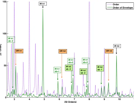
The most significant signatures used for bearing analysis were orders representations of two types of envelopes, namely envelope of a band pass filtered signal and the envelope of the de-phased signal (R. Klein et. al.). As can be observed in Figure 13 in the orders of the envelope of the de-phased signal the peaks related to the bearing failure modes are visible while in the regular orders representation the peaks are masked by the other rotating components excitation of higher energies.

2.1 Envelope of the filtered signal

An elevated frequency region at 7-10.5 KHz (in most cases separated from the high harmonics of the gear peaks) was identified as enhancing the bearing tones.

The identification of the frequency region was based on the visual inspection of the frequency PSD and the kurtogram of the wavelets decomposition of the raw signals. More details can be found in Sawalhi et. al., Antoni et. al., and Yang et. al. (2004).

The signal was band pass filtered around these frequencies, and then resampled according to the input shaft rotating speed. The envelope e(t)of the signal x(t) is the absolute value of the analytic signal e(t) x(t) jH

 

2.2 Envelope of the de-phased signal

The de-phase algorithm removes the phase averages (synchronous average) of all the shafts from the resampled signal, isolating the asynchronous excitations in the vibrations signal. The demodulated asynchronous excitations are represented by the spectra of the envelope of the de-phased signal (Klein et. al.).

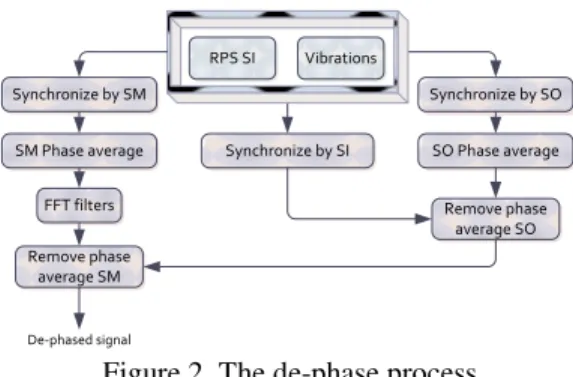
The de-phase process was performed in 5 stages (see Figure 2):

1. Generation of the phase average of the idler shaft (SM); 2. Generation of the phase average of the output shaft (SO); 3. Filtration of harmonics of the input shaft out from the

phase average of the output shaft using an ideal FFT band stop comb filter (removal of the harmonics of the input shaft coinciding with the multiples of 5 of the output shaft);

4. Resampling of the raw data according to the input shaft (SI);

5. Removal of the phase averages from the resampled data. The envelope was generated using the Hilbert transform and its spectrum was calculated.

The quality of the signatures obtained depends on the capability to isolate and remove the synchronous vibrations excitations, i.e. the quality depends on the phase average quality. In the PHM case we had some factors which made it easier to estimate the phase average signals, namely an accurate RPS measurement and vibrations acquisition during steady states. The main problems were due to the fact that the record length that were too short (especially considering the low RPS recordings) to allow enough averages for excitation sources separation.

Synchronize by SI Synchronize by SM

SM Phase average

Remove phase average SM

Vibrations RPS SI

FFT filters

Synchronize by SO

SO Phase average

Remove phase average SO

De-phased signal

Figure 2. The de-phase process

2.3 Bearing tones

Each time a contact with the damaged bearing surface occurs a shock is excited.

The repetition rate of the shocks with respect to the shaft rotating speed represents the rate of contacts of the damaged surface with other rolling elements. The rate of contacts on each type of surface (outer race, inner race, rolling elements, or cage) depends on the bearing geometry and the rotating speed of the inner and/or outer race. These rates of shocks characterize the damaged bearing and its failure mode. Assuming no slip between surfaces, the kinematic rates of contacts, i.e. Ball Pass Frequency Inner Race (BPFI), Ball Pass Frequency Outer Race (BPFO), Ball Spin Frequency (BSF), and the Fundamental Train Frequency (FTF), were calculated (see Table 1, Klein et. al., and McFadden et. al. (1990, 1984)).

3 the cage (FTF) and the rate of contacts with the damaged

ball will be twice the ball spin frequency (BSF).

The pointers by SI orders (multiples of the rotating speed of the input shaft) for the bearings are listed in Table 1, including pairs of bearings on the input shaft (BI), bearings on the idler shaft (BM), and bearings on the output shaft (BO).

BPFI RPS BPFO BSF 2BSF FTF BI 4.948 1 3.052 1.992 3.984 0.382 BM 1.648 1/3 1.019 0.664 1.329 0.042 BO 0.989 0.2 0.611 0.399 1.797 0.015 Table 1: Bearing tones and pointers in orders of the input

shaft (SI)

In order to differentiate between the bearing tones and the other peaks excited by other rotating components (gears and shafts) and in order to emphasize the expected patterns of peaks generated by damaged bearings the highest possible resolution is required.

2.4 High resolution spectra

As can be seen in Table 1, the separation of BO bearing tones would require a resolution of ~0.005 SI-orders, the separation of BM bearing tones would require a resolution of ~0.01 SI-orders, and the separation of BI bearing tones would require ~0.02 order by SI. With records of 2 sec. the maximum resolution that can be obtained while keeping a reasonable SNR (averaging enough FFT frames) is of 0.031 SI-orders.

The resolution of the spectra, Welch's PSD estimate – Pxx in Eq. (1), was improved using a procedure developed especially for the PHM challenge allowing the averaging of several (N) periodograms, X_i in Eq. (1), calculated with a resolution of 0.016 SI-orders. Instead of dividing the time series data into overlapping segments, computing a modified periodogram of each segment, and then averaging the PSD estimates, the averaging was performed on periodograms corresponding to different records that were classified as similar.





 N

i i

xx X

N P

1 2

1

(1) The similar records have been determined based on the results of hierarchical clustering. The algorithm for clustering of similar recordings had as inputs the orders by SI representation and the orders of both envelopes, of the filtered signal and of the de-phased signal. All the recordings having cophenetic distances below 65 were considered similar. The results of the hierarchical clustering were validated by other similarity checks and visual inspection.

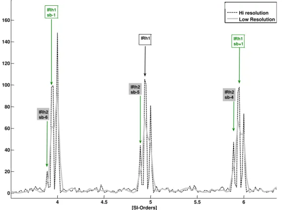
With the high resolution obtained the capability to isolate the damaged bearings on input shaft (SI) and in some cases on the idler shaft (SM) was improved. The comparison of results for a specific recording with a damaged bearing on the input shaft is illustrated in Figure 12. In the high resolution spectrum the peaks representing the faulty bearing (BPFI and the corresponding sidebands) have higher levels and are separated from the integer orders enabling the distinction of sidebands of different harmonics of BPFI.

2.5 Bearing features

The bearing tones derived from the bearing geometry may be inaccurate due to variations in the contact angle (axial loading) and due to slippage. In the orders domain, when the bearing tones are shifted the entire pattern of each harmony is shifted while the sidebands remain at the same distances. Therefore a special algorithm that searches and identifies the pointer location by pattern was applied. The algorithm for bearing feature extraction is using a reference signature (the respective baseline) in order to determine the location of the bearing‟s pointers.

The algorithm applies a comb filter representing the searched pattern (applied for each failure mode separately) and calculates the most probable location of the bearing tone and the median of the Mahalanobis distance of the entire pattern from the baseline population. The energies of the peaks above the background are then calculated completing the feature extraction for bearings.

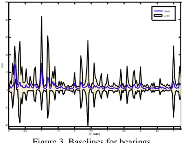
Initially a reference signature was created for each group of recordings at a certain nominal rotating speed based on the 15th percentile of the levels of the orders representations of the envelopes. Using this reference, the features of bearing failure modes have been extracted, and several recordings without damaged bearings were selected at each nominal rotating speed. In the second stage groups of 8-16 recordings were selected at each rotating speed and the baseline signature statistics were estimated (see Figure 3).

0 0.5 1 1.5 2 2.5 3 3.5 4 4.5 5

-40 -20 0 20 40 60 80 100

[SI-order]

none

mean ±3

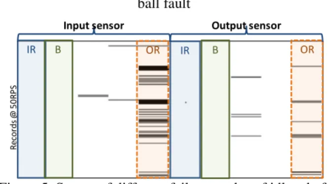
4 The results of the feature extraction of bearings on the input

shaft are displayed in Figure 4 and the results for bearings on the idler shaft are displayed in Figure 5. The figures represent the scores of the different failure modes of the bearings (the median of the Mahalanobis distance of the peaks with respect to the baseline). The scores of the bearings on the output shaft are not displayed because no damaged bearings have been detected.

R

e

cor

ds

@

50

R

P

S

IR B OR IR B OR

Input sensor Output sensor

Figure 4. Scores of different failure modes of input shaft bearings, IR – inner race fault, OR – outer race fault, B –

ball fault

R

e

cor

ds

@

50

R

P

S

IR B OR IR B OR

Input sensor Output sensor

Figure 5. Scores of different failure modes of idler shaft bearings, IR – inner race damage, OR – outer race damage,

B – ball damage

The algorithm detected only inner race and outer race damages of the bearings on the input shaft and only outer race damages of the bearings on the idler shaft. In several cases the same failure mode was detected on both sensors.

2.6 Bearing Decisions

The reasoning behind bearing decisions was similar for all bearings and failure modes.

In the cases where the scores (Mahalanobis distances from the baseline) were exceptionally high both in the envelope of the filtered signal and in the envelope of the de-phased signal and the pointer location was not an exact multiplier of one of the shaft speeds, we calculated the total energy of all the pointers in the pattern over 2-3 harmonies (including sidebands if relevant). The energies were extracted from the PSD of the envelope of the de-phased signal.

The total energies calculated per sensor were compared and in cases of clear discrimination the respective higher energy side (input side or output side) was diagnosed as having a

damaged inner/outer race or ball. The levels comparison is based on the assumption that the transmission path from each bearing to the adjacent sensor is similar. This assumption may not hold in practice.

In some recordings we observed very high levels of bearing tones on both sensors. These may be generated by combinations of faults, e.g. a bent or unbalanced input shaft and a damaged bearing, or two damaged bearings on the input shaft, or even high loads. We assumed that both bearings on the same shaft cannot have the same failure mode. In order to discriminate between these cases marked examples with faulty bearings are required for thresholds tuning.

In some cases peaks were observed and detected by the feature extraction algorithm at exact multiples of the shaft speeds (up to one point of the spectrum resolution). These cases were ignored in the decision process because they may be generated by modulation of faulty gears. The capability of both the filter and the de-phase algorithms to separate between the gears and bearings excitations was imperfect in this case: the de-phase algorithm capabilities were limited due to the short recordings (especially at low rotation speeds), and the envelope of the filtered signal was contaminated by faulty gears effects (at high rotation speeds). It seems, though, that the de-phase envelope has better capability to isolate the bearing excitations.

Another unknown was whether it was correct to ignore the patterns observed with low levels. When the sensor is located close to the damaged bearing and the excitations from other rotating components are relatively low, it can be that the bearing tones may be observed even when the bearing is in good condition. However, since we do not have such experience (maybe due to the complexity of the machinery that we usually diagnose), we did not know if that is the case here.

3 GEAR ANALYSIS

The most widely used signatures in gears analysis are in the orders, quefrency of orders and cycle domains (respectively equivalent to frequency, quefrency and time domains). The time history is mapped to the cycles‟ domain after synchronization (resampling) according to the rotating speed of a shaft.

The cepstrum of the orders representation was generated. The cepstrum reflects the repetition rate of sidebands (due to frequency modulation) and their average level in several peaks in the quefrency of orders domain (Zacksenhouse et. al., Antoni et.al.).

5 of the relevant shaft. The phase average signal reveals the

vibration induced by the meshing of each tooth on the relevant gear.

The phase average removes the asynchronous components by averaging the resampled signal in each cycle of rotation. All the signal elements that are not in phase with the rotation speed are eliminated, leaving the periodic elements represented in one cycle, i.e. the elements corresponding to harmonics of the shaft rotating speed.

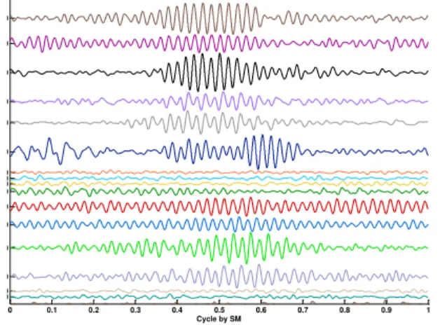
Phase average with frequency f is designed to remove elements in



representing a single cycle. The phase average capability to filter out the asynchronous elements depends on the number of cycles averaged (in this case M). Therefore, it is preferable to average over as many cycles as possible, i.e. over a long period of time. In the case of the PHM recordings the number of cycles averaged differed pending on the shaft rotating speed. For the input shaft the number of averages was 60-100 depending on the rotating speed. The number of averages for the idler shaft was in the range 20-33 and for the output shaft it was in the range of 12-20 (for SI RPS of 30-50Hz respectively). Therefore, the capability to filter out the asynchronous elements (in our case the bearing effects) was limited and the phase averages were more noisy than usual. In Figure 6 we can see a sample of phase average signatures filtered around the first harmonic of the gearmesh of a wheel (idler shaft at the output side – spur gears configuration).

0 0.1 0.2 0.3 0.4 0.5 0.6 0.7 0.8 0.9 1

50 50 50 50 50 50 50 50 50 50 50 50 50 50 50 50

Cycle by SM

Figure 6. Examples of phase averages filtered around the first harmonic of the spur output gear (SM cycle) Detection of abnormal meshing of individual teeth was achieved by further processing of the averaged signal into three types of signals: regular, residual, and difference (Zacksenhouse et. al.). The regular signals are obtained by passing the phase averaged signal through a multi-band-pass

filter, with pass-bands centered at the meshing frequency and its harmonics (1÷5). It is essentially the cycle-domain average of the vibrations induced by a single tooth. The residual signals are obtained by removing the meshing frequency harmonics. The difference signals are obtained by removing the meshing frequencies and adjacent sidebands, i.e. separating between the frequency and amplitude modulations.

The envelope and the unwrapped phase of the regular, difference and residual parts of all the harmonics describe the characteristics of the amplitude modulation.

3.1 Gear Features

Generally, the phase average is dominated by the gear meshing components and some low-order amplitude modulation and/or phase modulation components. These modulation effects are generated by transmission errors related to geometric and assembly errors of the gear pairs. When a localized gear fault is present, a short period impulse will appear in each complete revolution. This produces additional amplitude and phase modulation effects. Due to its short period nature, the impulse produces high order low-amplitude sidebands surrounding the meshing harmonics in the spectrum. The removal of the regular gear meshing harmonics (residual part) sometimes with their low-order sidebands (difference part) from the phase average emphasizes the portion predominantly caused by gear fault and geometrical and assembly errors. Statistical measures of the residual part were used to quantify the fault-induced shocks.

Orders representation of the phase average according to each shaft was generated. The peak values at each harmonic of the shaft rotating speed representing gearmesh orders and sidebands were stored as features characterizing the gears. The features of gears were extracted both for the spur and helical configurations. The features extracted for each gear wheel included: the even un-normalized statistical moments (RMS, kurtosis, 6th and 8th moments) of the regular, residual and difference parts, the even moments of the envelope of the regular, residual and difference, the peak values of the orders representation of the phase average for the gearmesh and the respective shaft sidebands, and the levels of the cepstrum representing the quefrency of the respective shafts. In the regular procedure these features are “normalized” to the baseline transforming the moments into the known features FM0, FM2, FM4, FM6, FM8, NA4, NB4, etc. (see Lebold et. al.) and in later stages the gears wheels scores are determined using Mahalanobis distances from the baseline features. This procedure was modified for the case of the challenge when the normalization process and the distances measurement were omitted.

N n

M y

M

m mN n

n 1, ,

1 :

1

0

 





 

6

3.2 Spur/ Helical Clustering

It is well known that spur gears generate higher vibrations levels compared to helical gears. Therefore one of the features selected for the gearbox configuration classification was the energy of the background of the frequency spectra. The background signature was selected in order to avoid influence of the damaged components. The background of the frequency spectra was estimated based on an adaptive clutter separation algorithm.

The other features used for classification included the ratios of the energies of the spur/helical gearmesh orders of the wheel on the output shaft and of the wheels on the idler shaft. Recordings with similar rotating speed were clustered (hierarchical clustering) and classified using the above features as spur or helical.

3.3 Gear Diagnostics

The numerous features extracted for each gear wheel (statistical moments of all the harmonics of the regular, residual and difference parts etc…) were “normalized” with respect to the population of the same type of machine (spur/helical) at the same speed (by normalization we mean calculation of the Mahalanobis distance). A matrix of these non-dimensional features of a gear wheel was displayed and the exceptional recordings were selected (see Figure 7). The discrimination between the different failure modes was based on automatic screening of features and visual inspection of the phase averages of the first harmonics and the sum of harmonics.

Envelope Phase PhA

Figure 7. Scores of output spur gear – recordings at 50 RPS. The left third represents harmonics 1-5 (and over-all) scores

of the envelope. The middle third represents the phase scores of harmonics 1-5 (and over-all), and the right third represents the phase-average scores of harmonics 1-5 and over-all. The scores of the idler gearwheel and output

gearwheel are alternating.

The distributed faults (error related to the teeth spacing) were revealed by the RMS of the first harmony in all the types of phase averaged signals. The high RMS levels were most emphasized in the envelope of the first harmonic. In the orders domain appearance of sidebands was observed mainly around the first harmonic.

The localized faults were emphasized in the higher harmonics in all the statistical moments and in all the parts of the phase average. In the orders domain numerous high orders sidebands were elevated.

The fault location in the case of one of the wheels on the idler shaft was decided based on the orders representation, the comparison of the sensors, and the effect on the meshing gears on the other shafts.

It should be pointed out that all the signatures and hence features described are affected by mechanisms associated with the cross-gear interference, i.e. the vibrations induced by one gear (gear meshing) are modulated by the vibrations of another gear (gear meshing). For instance, in the PHM apparatus, a fault in the input pinion gear may cause a modulation of the pinion tooth meshing frequency with the tooth meshing of the large gearwheel, resulting in an erroneous identification of the fault location. Demodulation is impractical in the PHM apparatus since the gear mesh orders are exact multiples.

3.4 An example of a Distributed Fault Diagnostics

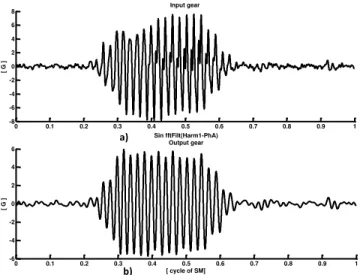
The diagnostic process of a distributed fault is illustrated using results from a recording classified as a spur gear at 50 RPS.

a) b)

c) d)

Figure 8. Phase averages of spur gear wheels from one recording with a faulty gear: a) input gearwheel, b) input

idler gearwheel, c) output idler gearwheel, and d) output gearwheel.

7 easily observed on both wheels on the idler shaft (SM)

while the amplitude is higher on the input gear wheel. In Figure 9 it can be seen that the phase average signal is less noisy on the output gearwheel of the idler shaft than on the input gearwheel of the same shaft.

0 0.1 0.2 0.3 0.4 0.5 0.6 0.7 0.8 0.9 1

-8 -6 -4 -2 0 2 4 6

8 Input gear

[ G

]

0 0.1 0.2 0.3 0.4 0.5 0.6 0.7 0.8 0.9 1

-6 -4 -2 0 2 4 6 Sin fftFilt(Harm1-PhA) Output gear

[ cycle of SM]

[ G

]

a)

b)

Figure 9. Phase averages of the first harmonic of spur gearwheels on the idler shaft. This example was taken from

a recording with a faulty gear. a) Input gearwheel and b) output gearwheel.

15 20 25 30 35

0 2 4 6 8 10 12

[ order by SI]

[ G^

2/o

rde

r ]

12 13 14 15 16 17 18 19 20 0 0.05 0.1 0.15 0.2 0.25 0.3 0.35 0.4 0.45 0.5

[ order by SI]

[ G^

2/o

rde

r ]

Figure 10. SI-Orders PSD of a spur gear recording with a faulty gear (grey) compared to a healthy gear (black) In order to identify the fault location we checked several criteria:

The influence on the meshing gear wheels: If the faulty gear wheel is on the input gear we would expect a higher impact on the gear wheel of the input shaft and the expected effect is a “smeared” envelope similar to the envelope on the faulty gear wheel. If the faulty wheel is on the output gear we would expect a signal with an envelope similar to the faulty gearwheel repeated 5 times. This can be observed in Figure 8.

The FM modulation represented in the orders domain: FM modulation is expected to appear more clearly around the gearmesh of a faulty gear. In the case of spur gears, if the faulty wheel is on the input gear we would expect to see it around SI-order 32, and in the case that the fault is on the wheel of the output gear, around SI-order 16. In our case the fault is clearly located on the output gearwheel (see Figure 10).

Inspecting the statistical moments of the phase average, residual, difference, and their complex envelopes (Figure 7) we can see that the faults are manifested especially in the second statistical moments of the envelope. Of these the most relevant are the moments of the first harmonic and the overall signals (1-5 harmonics, see Figure 11).

1st_{harmonic 2}nd_{harmonic 3}rd_{harmonic 4}th_{harmonic 5}th_{harmonic All harmonics}

PhA

D R D R PhA D R PhA D R PhA D R PhA D R PhA S M S O S M S O S M S O S M S O S M S O S M S O S M S O S M S O S M S O S M S O S M S O S M S O S M S O S M S O S M S O S M S O S M S O S M S O Fa u lt y g e a r

Figure 11. Second order statistical moments of the envelopes of: phase average (PhA), residual (R), and difference (D); harmonics 1-5 and over-all of alternating idler and output gearwheels. The lower four rows represent

faulty idler gearwheels.

4 SHAFT ANALYSIS

The orders representation of the phase average according to each shaft is the most significant signature in the shaft analysis.

4.1 Shaft features

The features extracted for the shafts were the peak values of the first 5 harmonics of the respective phase average signals.

4.2 Shaft diagnostics

Unbalance of the input shaft was diagnosed based on the shaft rotating speed (1st order).

8

5 CONCLUSIONS

Spectra in the frequency and orders domains did not always reveal the bearing faults. However, failures of the bearings are detectable by either envelope of the de-phased signal and envelope of the signal filtered around resonance frequencies.

Fault localization on similar bearings on the same shaft (in the PHM challenge case, discrimination between the input and output side bearings on a shaft) is problematic without marked cases of healthy and faulty bearings.

Detection of bearing faults requires high resolution (which for a given bandwidth can be obtained with longer recording time).

Detection of bearing faults requires wide-band data regardless of the fact that commonly the pointers are at low frequencies (the resonance frequencies enhancing the bearing tones are much higher than the rate of shocks representing the contact with the damaged surface).

De-phase process performs well under steady-state conditions and allows enhanced bearing detection even if the number of averages is low.

The diagnostics of bearings can be achieved using fully automatic algorithms.

Distributed gear failures are detectable using statistical moments of the envelope of the phase average, residual and difference signals (especially around first gearmesh harmony).

Correct classification of operation conditions can greatly improve reliability of diagnostics. In the PHM case, operation conditions were uncertain due to unmarked load variations (high, low, bad key).

Automatic localization of the faulty gear wheel is challenging due to the fact that wheels on the same shaft are indistinguishable. Cross-gear interference may lead to erroneous identification of faults.

NOMENCLATURE

e(t) envelope of the signal FM Frequency Modulation H{} Hilbert transform PhA Phase Average Pxx Welch's PSD estimate R residual signal D difference signal PSD Power Spectral Density RMS Root Mean Square RPS Rotations Per Second [Hz] SI input shaft rotating speed SM idler shaft rotating speed

SO output shaft rotating speed

) (t

x signal

REFERENCES

Antoni J. & Randall R. B. (2002), Differential Diagnosis of Gear and Bearing Faults, Journal of Vibration and Acoustics, Vol. 124,pp165-171.

Azovtsev A. & Barkov A. (1984), Rolling Element and Fluid Film Bearing Diagnostics Using Enveloping Methods, Vibro Acoustical Systems and Technologies, Inc.

Klein R., Rudyk E., Masad E. & Issacharoff M. (2009), Emphasizing bearings‟ tones for prognostics, The Sixth International Conference on Condition Monitoring and Machinery Failure Prevention Technologies, pp. 578-587.

Lebold M., McClintic K., Campbell R., Byington C. & Maynard K. (2000), Review of vibration analysis methods for gearbox diagnostics and prognostics, Proceedings of 54th Meeting of the Society for Machinery Failure Prevention Technology, Virginia Beach, VA, May 1-4, 2000, pp. 623-634.

McFadden P. D. & Smith J. D. (1984, February), Vibration Monitoring of rolling element bearing by the high-frequency resonance technique - a review, Tribology international, Vol 17, pp 3-10.

McFadden P. D. (1990), Condition monitoring of rolling element bearing by vibration analysis, Proceedings of the Inst. Mech. Eng., Seminar on machine condition monitoring, pp 49-53, 1990.

Sawalhi N. & Randall R. B., Semi-automated bearing diagnostics – three case studies, School of Mechanical and Manufacturing Engineering, The University of New South Wales, Sydney, Australia.

Wang Y. F. & Kootsookos P. J. (1998), Modeling of Low Shaft Speed Bearing Faults for Condition Monitoring, Mechanical Systems and Signal Processing, 12(3) pp 415-426.

Yang W. X. & Ren X. M. (2004), Detecting Impulses in Mechanical Signals by Wavelets, EURASIP journal on Applied Signal Processing, pp 1156-1162.

Zacksenhouse M., Braun S., Feldman M. & Sidahmed M. (2000), Toward Helicopter Gearbox Diagnostics from a Small Number of Examples, Mechanical Systems and Signal Processing, 14(4) pp 523-543.

Renata Klein received her B.Sc. in Physics and Ph.D. in the

9 and prognostics systems that are used successfully in

combat helicopters of the Israeli Air Force, in UAV‟s and in jet engines. Renata was a lecturer in the faculty of Aerospace Engineering of the Technion, where she developed and conducted a graduate class in the field of machinery diagnostics. In the last three years, Renata is the CEO and owner of “R.K. Diagnostics”, providing R&D services and algorithms to companies who wish to integrate Machinery health management and prognostics capabilities in their products.

Eduard Rudyk holds a B.Sc. in Electrical Engineering

from Ben-Gurion University, Israel, M.Sc. in Electrical Engineering and MBA from Technion, Israel Institute of Technology. His professional career progressed through a series of professional and managerial positions, leading development of pattern recognition algorithms for medical

diagnostics and leading development of health management and prognostics algorithms for airborne platforms, such as UAV‟s and helicopters. For the last 2 years Eduard is the director of R&D at "R.K. Diagnostics".

Eyal Masad received his B.Sc., M.Sc. and Ph.D. degrees

from the Faculty of Mathematics in the Technion, Israel Institute of Technology. His research topics were in the fields of Machine learning, Information theory, nonlinear analysis and topological dynamics. In the last two years, Eyal is an algorithms developer at “R.K. Diagnostics”.

Moshe Issacharoff holds a B.Sc. in Electrical Engineering from the Technion, Israel Institute of Technology. Moshe started his professional career in ADA-Rafael, the Israeli Armament Development Authority. During the last 2 years Moshe is an algorithms developer at "R.K. Diagnostics".

4 4.5 5 5.5 6

0 20 40 60 80 100 120 140 160

[SI-Orders]

Hi resolution Low Resolution

IRh2 sb-5

IRh2 sb-6

IRh1

IRh1 sb-1

IRh2 sb-4

IRh1 sb+1

Figure 12. Comparison of low resolution (solid grey) and high resolution (dashed) of the orders by SI of the envelope of the de-phased signal. IR patterns of various harmonies are visible in the high resolution (h stands for harmony and sb stands for

10

3 4 5 6 7 8 9 10 11

0 50 100 150

[SI Orders]

[G

2/Or

der

]

Order

Order of Envelope IR h1

IR h2

IR h1 sb+1

IR h1 sb+2

IR h1 sb+3 IR h1

sb -2

IR h2

sb -3 _{IR h2} IR h2sb -1 sb -2

OR h1 OR h2 OR h3