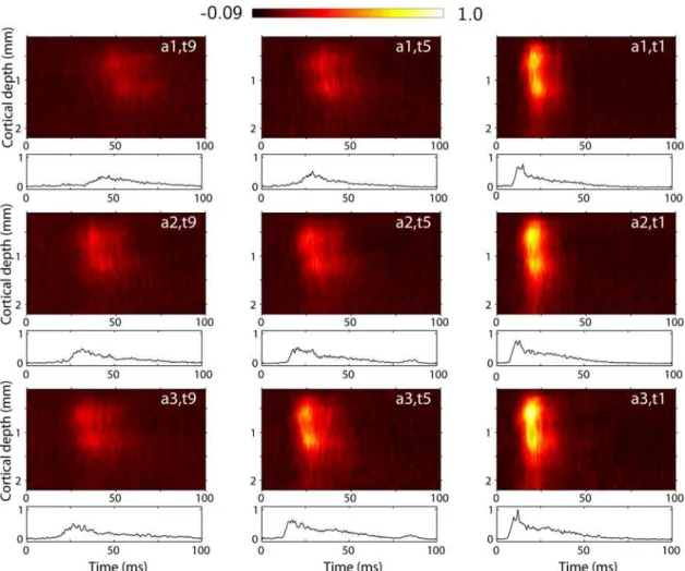
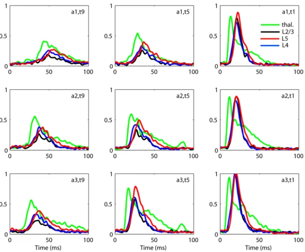
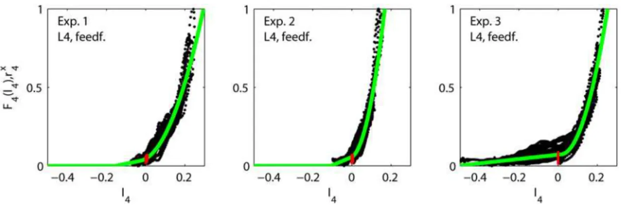
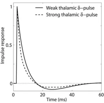
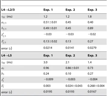
Estimation of thalamocortical and intracortical network models from joint thalamic single-electrode and cortical laminar-electrode recordings in the rat barrel system.

Peça de mão de alta rotação pneumática com sistema Push Button (botão para remoção de broca), podendo apresentar passagem dupla de ar e acoplamento para engate rápido

Neste trabalho o objetivo central foi a ampliação e adequação do procedimento e programa computacional baseado no programa comercial MSC.PATRAN, para a geração automática de modelos

Ousasse apontar algumas hipóteses para a solução desse problema público a partir do exposto dos autores usados como base para fundamentação teórica, da análise dos dados

Em sua pesquisa sobre a história da imprensa social no Brasil, por exemplo, apesar de deixar claro que “sua investigação está distante de ser um trabalho completo”, ele

Isto é, o multilateralismo, em nível regional, só pode ser construído a partir de uma agenda dos países latino-americanos que leve em consideração os problemas (mas não as

Despercebido: não visto, não notado, não observado, ignorado.. Não me passou despercebido

Caso utilizado em neonato (recém-nascido), deverá ser utilizado para reconstituição do produto apenas água para injeção e o frasco do diluente não deve ser

O presente trabalho teve por objetivo a determinação da área de forrageamento e a estimativa da população de uma colônia de Heterotermes tenuis com posterior avaliação da