www.geosci-instrum-method-data-syst.net/5/567/2016/ doi:10.5194/gi-5-567-2016
© Author(s) 2016. CC Attribution 3.0 License.
Application of ground-penetrating radar technique to
evaluate the waterfront location in hardened concrete
Isabel Rodríguez-Abad1, Gilles Klysz2, Rosa Martínez-Sala1, Jean Paul Balayssac2, and Jesús Mené-Aparicio1
1Universitat Politècnica de València, Camino de Vera s/n, Valencia, 46022, Spain 2LMDC, Université de Toulouse, INSAT, UPS, Toulouse, France
Correspondence to:Isabel Rodríguez-Abad ([email protected])
Received: 30 June 2016 – Published in Geosci. Instrum. Method. Data Syst. Discuss.: 4 August 2016 Revised: 14 November 2016 – Accepted: 15 November 2016 – Published: 15 December 2016
Abstract. The long-term performance of concrete struc-tures is directly tied to two factors: concrete durability and strength. When assessing the durability of concrete struc-tures, the study of the water penetration is paramount, be-cause almost all reactions like corrosion, alkali–silica, sul-fate, etc., which produce their deterioration, require the pres-ence of water. Ground-penetrating radar (GPR) has shown to be very sensitive to water variations. On this basis, the ob-jective of this experimental study is, firstly, to analyze the correlation between the water penetration depth in concrete samples and the GPR wave parameters. To do this, the sam-ples were immersed into water for different time intervals and the wave parameters were obtained from signals regis-tered when the antenna was placed on the immersed surface of the samples. Secondly, a procedure has been developed to be able to determine, from those signals, the reliability in the detection and location of waterfront depths. The results have revealed that GPR may have an enormous potential in this field, because excellent agreements were found between the correlated variables. In addition, when comparing the water-front depths calculated from GPR measurements and those visually registered after breaking the samples, we observed that they totally agreed when the waterfront was more than 4 cm depth.
1 Introduction
Concrete is the most used man-made construction material around the world. For this reason, the durability of the con-crete structures plays an important role when trying to avoid repairs and replacements, which in turn reduces costs and
environmental impacts. The traditional systems used to as-sess the durability of concrete structures are expensive, time consuming and, what is worse, cause damages. To overcome these drawbacks, nondestructive techniques (NDTs) are be-ing under study to measure concrete properties that are re-lated to durability.
The long-term performance of concrete structures can be compromised not only by poor construction practices but also, due to the permeability of concrete, by environmen-tal agents, when they are aggressive. Since concrete is a porous material, water, containing dissolved potential delete-rious substances or gases, may penetrate and be transported through the pore structure and cracks. Later on, the presence of moisture may contribute to the chemical and physical de-terioration of the concrete. In particular, for much pathology, the common catalyst is moisture, since all chemical reac-tions (corrosion, alkali–silica, sulfate, etc.) need some water to develop (Klysz et al., 2008). Therefore, the analysis of wa-ter penetration in concrete is critical when durability studies are performed (Otieno et al., 2010)
Currently there are several NDTs available to evaluate the condition of structures from the effects of moisture pene-tration. Tosti and Slob (2015) give a quick review about those methods and highlight the big potential of ground-penetrating radar (GPR).
Figure 1. (a)Concrete samples immersed into 3 cm of water;(b)GPR acquisition procedure;(c)waterfront marked in the sample after conducting GPR measurements and breaking the sample.
et al., 2009). Previous studies have reported the effect of wa-ter content on wave paramewa-ters. Some of them (Laurens et al., 2005; Sbartaï et al., 2006; Klysz and Balayssac, 2007; Martínez-Sala et al., 2013) have shown the suitability of the direct signal attenuation to characterize water content in con-crete. Other works analyze the influence of water content on waves energy (Martínez-Sala et al., 2015) and models have been developed to prove a strong correlation between radar amplitude attenuation and the moisture content (Senin and Hamid, 2015; Klysz et al., 2008). A review about the tech-niques based on time domain and frequency on radar signals is provided by Tosti and Slob (2015). However, as far as we know, the studies carried out by Rodríguez-Abad et al. (2014, 2016a) are the only ones that deal with the assessment of the location and determination of the waterfront depth from elec-tromagnetic wave parameters.
In line with this former investigation, the aim of this paper is to analyze the effect of differential waterfront depths on the wave velocity and find out the waterfront depth in con-crete specimens, which have been partially immersed in wa-ter. While the study of Rodríguez-Abad et al. (2016a) was conducted placing the GPR on the surface opposite the im-mersed one, in this case, the study was performed by plac-ing the GPR antenna on the same surface that was immersed into water, the preliminary analysis of which was presented in the European Geosciences Union (EGU) General Assem-bly (Rodríguez-Abad et al., 2016b). To carry out these two studies, 24 concrete specimens were fabricated, cured and dried in a kiln. After being partially immersed in water dur-ing different time intervals, for the present work, GPR mea-surements were conducted on the wet face of the samples by using a 2 GHz antenna. Finally, the samples were broken to visually measure the actual waterfront depth.
2 Material and method
The experimental program was conducted on ordinary con-crete samples made with water / cement ratio of 0.65, manu-factured with a CEM I 52,5 R/SR cement. A total of 24 con-crete samples measuring 0.20×0.20×0.12 m3 were fabri-cated. The samples were cured by immersion in a wet cham-ber for a period of 28 days, in accordance with the
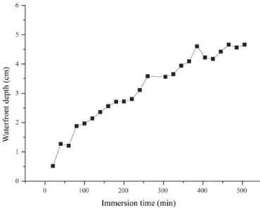
stan-Figure 2.Waterfront depth advance in time.
dard (UNE-EN 12390-2:2009). After that, they were left to conduct the curing process under atmospheric conditions up to 90 days. With this age the samples were introduced in a kiln (105◦
C) to dry them completely. Subsequently, the sam-ples were taken out of the kiln and sealing paint was applied on all surfaces, except for the ones that would be in contact with water and the opposite side. Finally, samples were im-mersed into 3 cm of water (Fig. 1a).
The GPR measurements were performed before and after submerging the samples. Finally, all specimens were broken in two parts and the correct positions of the waterfronts were marked and measured. The final waterfront values are de-picted in Fig. 2. By means of the visual inspection, it could be clearly observed that the distribution consisted of a satu-rated zone and a drier zone (Fig. 1c).
Figure 3.Effect of water immersion on reflected peaks.
3 Results and discussion
3.1 Effect of water content on direct and reflected wave GPR signals
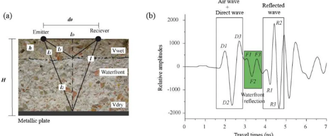
Prior to performing any measurements in the GPR signals, it was necessary to understand the received signals. They were composed by two parts: the direct wave, considering this one as the overlap between the air wave and the direct wave, and the reflected wave at the bottom of the samples. Both of them were composed by three main peaks, respectively (D1, D2, D3, R1, R2, R3) and were affected by the water immersion (Fig. 3).
To calculate the propagation velocities, it was necessary to measure the arrival times in GPR signals. However, due to the interference and the attenuation of the waves, it was difficult to identify which maximum was representative of the wave arrival. To overcome this difficulty, velocities were calculated with all the peaks combinations in order to know which one provided better agreement with the waterfront depth. For each sample and peak combination, the velocity was calculated with the following equation:
v= 2l 1tDR=
2
r
H2+d0 2
2!
1tDR , (1)
where l was the half of the path the wave traveled, 1tRD was the arrival time increment between the reflected and di-rect wave,d0was the distance between emitter and receiver
(4 cm) and Hthe width of the sample (12 cm). Finally, the velocity difference, when the sample was dry and wet, was determined by Eq. (2):
1v cm
ns
=vim−vd, (2)
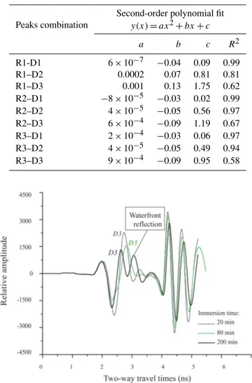
Table 1.Waterfront advance depth in centimeters and best adjust-ments with velocity increadjust-ments.
Peaks combination
Second-order polynomial fit
y(x)=ax2+bx+c
a b c R2
R1-D1 6×10⁻⁷ −0.04 0.09 0.99
R1–D2 0.0002 0.07 0.81 0.81 R1–D3 0.001 0.13 1.75 0.62 R2–D1 −8×10⁻⁵ −0.03 0.02 0.99 R2–D2 4×10⁻⁵ −0.05 0.56 0.97
R2–D3 6×10⁻⁴ −0.09 1.19 0.67 R3–D1 2×10⁻⁴ −0.03 0.06 0.97
R3–D2 4×10⁻⁵ −0.05 0.49 0.94 R3–D3 9×10⁻⁴ −0.09 0.95 0.58
Figure 4.Overlap between peak D3 of direct wave and waterfront reflection.
wherevim was the wave velocity when the sample was
im-mersed into water andvdwas the velocity when the sample
was dry.
In addition, velocity increments were correlated with the waterfront depths in order to check which one provided a bet-ter agreement between both paramebet-ters. The results of which are summarized in Table 1.
The results show a good agreement between velocity in-crements and waterfront depth for all peaks combinations, except for the ones that were calculated with peak D3. This result was expected, since D3 was a peak affected by two sig-nals: the direct wave and the reflection of the waterfront. It is not after 325 min of immersion that the waterfront reflection was totally separated from the direct wave (Fig. 4).
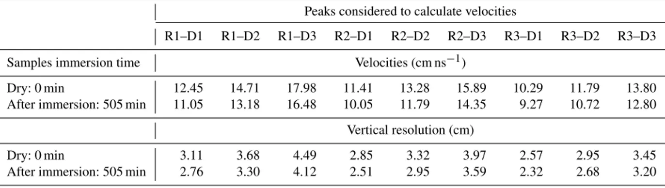
re-Table 2.Theoretical vertical resolution, considering the different peaks combinations to calculate velocities.
Peaks considered to calculate velocities
R1–D1 R1–D2 R1–D3 R2–D1 R2–D2 R2–D3 R3–D1 R3–D2 R3–D3 Samples immersion time Velocities (cm ns−1)
Dry: 0 min 12.45 14.71 17.98 11.41 13.28 15.89 10.29 11.79 13.80 After immersion: 505 min 11.05 13.18 16.48 10.05 11.79 14.35 9.27 10.72 12.80
Vertical resolution (cm)
Dry: 0 min 3.11 3.68 4.49 2.85 3.32 3.97 2.57 2.95 3.45 After immersion: 505 min 2.76 3.30 4.12 2.51 2.95 3.59 2.32 2.68 3.20
liability, regardless of the peaks combination used, except for D3. In particular, the peaks combination of D1–R1 used to calculate the velocity increment presented an excellent cor-relation, as can be observed in Fig. 5.
3.2 Effect of waterfront reflection on GPR signals The next step was to process the waterfront reflection. Ac-cording to Pérez Gracia (2001) the vertical resolution (Rv) is
calculated by the following equation: Rv=
v
2f, (3)
where v is the wave velocity and f is the wave frequency. In Table 2 the extreme velocity values and vertical resolu-tion are presented, which ranged from 2.3 to 4.5 cm. This means that interfaces located under these distances might not be identifiable. Nevertheless, the following analysis was con-ducted to check the reliability of this statement.
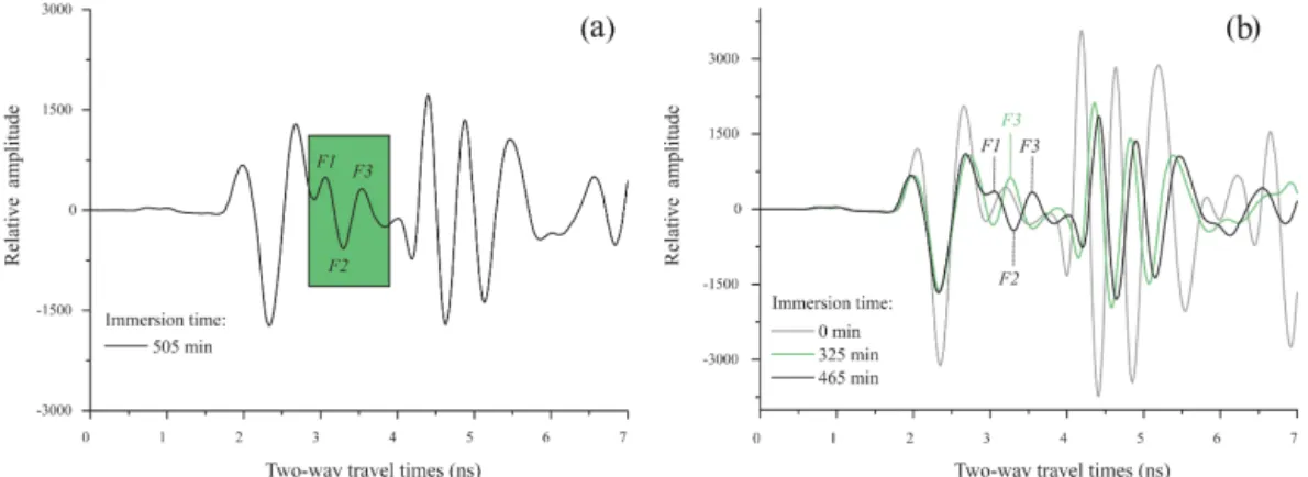
The waterfront reflection was composed of three maxi-mums (F1, F2 and F3), but they were only identifiable af-ter a long period immersed in waaf-ter (465 min), as it can be observed in Fig. 6. Only after 325 min of immersion, the wa-terfront reflection was not overlapped with the direct wave and as the waterfront depth increased its signal become more easily identifiable. Nevertheless, in all cases the peak F3 was reliably identifiable; therefore, it was used as the waterfront reflection arrival in the following calculations.
In order to check the reliability of the waterfront iden-tification, a regression linear analysis was used to find the relationship between the arrival times of the direct and re-flected peaks and the waterfront peaks. As it can be observed in Fig. 7, an excellent agreement was found between peak D2 of the direct wave and F3 of the waterfront reflection. Like-wise, excellent results were found when relating peak R3 of the reflected wave and F3 of the waterfront.
These results are of great importance, because that means that the GPR technique working with a commercial antenna of 2 GHz central frequency had enough sensitivity to detect a waterfront that ranged from 0.5 to 4.7 cm and this limit was far beyond the theoretical vertical resolution (Table 2).
Figure 5.Velocity increments calculated with the peaks combina-tion D1–R1 versus waterfront depth.
3.3 Waterfront depth assessment
The final step was to assess the capability of GPR signals to determine the waterfront depth. Although there is refraction at the interface between dry and wet concrete, in this work we use a simpler model. Due to the small sample size, the short distances of the propagation paths and the refraction angle changes, we consider them to be neglected. Consider-ing this approach, this model is depicted in Fig. 8. AnalyzConsider-ing propagation paths, arrival time increments at the different in-terfaces reflections were able to be calculated. The equations of these time increments were
h (1t )R1D2i
wet
=2
l1 vwet
+ l2 vdry
− d0 vwet
, (4)
h (1t )R3F3i
wet
=2
l1 vwet
+ l2 vdry
− l3 vwet
, (5)
where (1t )R1D2wet were arrival time increments between direct and reflected at the bottom of samples waves and
Figure 6. (a)Waterfront reflection maximum peaks;(b)waterfront reflection evolution along immersion time.
Figure 7. (a)Adjustments of the arrival time increment between D2 and waterfront reflection (F3) and waterfront depths;(b)arrival time increment between R3 and waterfront reflection (F3) and waterfront depths.
were possible to be measured in the GPR signals. Likewise, vdry, which corresponds to the velocity of the GPR signals
along the dry part of samples, was calculable from the GPR signals by means of the following equation:
vdry=
2
r
H2+d0 2
2!
1tD2R1 dry
, (6)
where 1tD2R1drywas the arrival time increments between re-flected and direct waves when samples were dry,d0was the
distance between emitter and receiver andHthe width of the sample. In addition, the half of the paths that each wave trav-eled, that is l,l1,l2 andl3 (Fig. 8), could be calculated as
follows:
l=
s d
0
2
2
+H2, (7)
l1= h
Hl, (8)
l2= H−h
H l, (9)
l3= s
d 0
2
2
+h2, (10)
wherehwas the unknown value to be determined: waterfront depth. Substituting Eqs. (6), (7), (8), (9) and (10) in Eqs. (4) and (5), we had two equations with two unknowns: water-front depth and velocity in the wet part of the sample (vwet).
Thevwet was assumed to be constant, since the absorption
coefficient of the wet zone remained quite stable (Average CA wet zone=4.5 %), regardless of the height of the
water-front.
After solving these two nonlinear equations system, the waterfront was determined. The solution did not converge for the first 325 min of immersion. This was expected, since some generalizations were assumed when calculating the propagation paths and, in addition, the waterfront depths of these samples were on the range of the antenna resolution. Nevertheless, very interesting results were obtained for the samples that remained immersed more than 345 min. The waterfront depths obtained after breaking the samples and the ones calculated by the procedure explained above are de-tailed in Table 3.
Figure 8. (a)Sketch of the propagation paths model;(b)typical GPR signal acquired when the sample was immersed.
Table 3.Waterfront determination by means of GPR signals.
Waterfront depth (cm) Sample
immersion After breaking GPR Difference time samples signals (cm) 345 4.04 3.35 0.69
365 4.17 – –
385 4.79 4.50 0.29 405 4.22 3.95 0.27 425 4.28 3.85 0.43 445 4.52 4.35 0.17 465 4.73 4.65 0.07 485 4.56 4.70 −0.14 505 4.67 4.75 −0.08
in contact with water, waterfront depths could be calculated quite accurately, but only when the waterfront had a height bigger than 4 cm.
4 Conclusions
Concrete durability depends mainly on its permeability. Therefore, the analysis of water penetration in concrete is critical when durability studies are performed. This research analyzed the capability of the GPR technique to evaluate the location of the waterfront by means of a commercial antenna of 2 GHz central frequency, when the GPR data were ac-quired placing the antenna on the surface of the concrete specimen which was immersed into water. The election of this antenna display was based on the idea that this will be probably the only possible acquisition procedure when studying concrete structures in service.
It was found that direct and reflected waves at the sam-ples bottom were greatly affected by the waterfront advance, since they described with great approximation the waterfront
increment. It is very important to highlight that it was not necessary to locate the waterfront reflection to find great cor-relations between these parameters (R2=99 %). In addition, despite the fact that the waterfront height was smaller than the vertical resolution, the location of the waterfront reflec-tion was possible after analyzing the GPR signals. Indeed, it was possible to detect the waterfront arrival, even in those cases in which the waterfront was overlapped with the di-rect wave, as it was proven by the high correlation coeffi-cients found (R2=99 %). Finally, a special procedure was developed to calculate the waterfront position. In this case, the results proved that by using the simplified model of the propagation paths used in this work, it was possible to assess the waterfront depth, although only when it was greater than 4 cm.
For all these reasons, it can be concluded that the GPR is a powerful technique to assess and locate the waterfront advance in hardened concrete when using a 2 GHz commer-cial antenna. However, further research will be needed with a larger number of samples, with a variety of dimensions and different water/cement ratios and different frequency anten-nas.
5 Data availability
Figure A1.Electromagnetic traveling paths models.
Appendix A: Justification of the approximations of the electromagnetic modeling
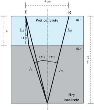
In Fig. A1, electromagnetic modeling (EM modelling A) that takes into account the bending of the propagation paths and the electromagnetic modeling used in this paper (EM model B) can be observed. The EM model B considers some approximations and their validity was justified by the following calculations.
The first step to validate EM model B was its definition. As depicted in Fig. A1, there were two media that corre-sponded to the wet (m1) and dry concrete (m2). EM model
B considered that there was no change in the propagation paths. Therefore, l1B and l2B was assumed to be a single
line. The second step was to calculate the length of l1Band l2B. According to the dimensions of the concrete samples
and the distance between emitter and receiver of the 2 GHz antenna manufactured by GSSI, the reflection angle in this model (α2B) was calculated as follows:
∝2B=arctg
2 12
=9.460. (A1) For the most unfavorable case, that is, when the waterfront was deepest, the waterfront depth (h) when the sample was broken was found to beh=4.70 cm (Table 3). Then,l1Band l2Bwere calculated with Eqs. (12) and (13).
l1B= h cos∝2B
=4.76 cm (A2)
l2B=
12−h cos∝2B
=7.40 cm (A3)
The third step was to calculate the length of the travel paths considering EM model A (l1Aandl2A). According to Snell’s
law and the geometry of the problem (Fig. A1), we obtained two equations with two unknowns:
v2 v1
=sinα2A sinα1A
, (A4)
(12−h)·tgα2A+h·tgα1A=2. (A5)
To solve Eqs. (14) and (15), the most unfavorable case (h=4.70 cm) was considered, in which the resulting velocities when solving the Eqs. (6) and (4) for this sam-ple were propagation velocity when the wave traveled along the wet part,v1=(vwet)R1D2=8.18 cm ns−1, and when
trav-eled along the dry part,v2= vdryR1D2=12.40 cm ns−1.
Fi-nally, the refraction angles were found to beα1A=7.18◦and α2A=10.92◦and the pathsl1Aandl2Awere calculated with
Eqs. (16) and (17). l1A=
h cos∝1A
=4.74 cm (A6)
l2A=
12−h cos∝2A
=7.43 cm (A7)
The Supplement related to this article is available online at doi:10.5194/gi-5-567-2016-supplement.
Acknowledgements. The authors are grateful to COST - European Cooperation in Science and Technology (www.cost.eu) for funding the Action TU1208 “Civil engineering applications of Ground Penetrating Radar” (www.GPRadar.eu). The authors also thank the Laboratorio de Materiales de Construción of the Escuela Técnica Superior de Ingeniería de la Edificación de la Universitat Politèc-nica de València techPolitèc-nical team for the valuable collaboration. Edited by: F. Soldovieri
Reviewed by: three anonymous referees
References
Klysz, G. and Balayssac, J. P.: Determination of volumetric water content of concrete using ground-penetrating radar, Cement Con-crete Res., 37, 164–117, doi:10.1016/j.cemconres.2007.04.010, 2007.
Klysz, G., Balayssac, J. P., and Ferrières, X.: Evaluation of dielec-tric properties of concrete by a numerical FDTD model of a GPR coupled antenna-Parametric study, NDT&E Int., 41, 621–631, doi:10.1016/j.ndteint.2008.03.011, 2008.
Lai, W. L., Kou, S. C., Tsang, W. F., and Poon, C. S.: Character-ization of concrete properties from dielectric properties using ground penetrating radar, Cement Concrete Res., 39, 687–695, doi:10.1016/j.cemconres.2009.05.004, 2009.
Laurens, S., Balayssac, J. P., Rhazi, J., Klysz, G., and Arliguie, G.: Non-destructive evaluation of concrete moisture by GPR: exper-imental study and direct modelling, Mater. Struct., 38, 827–832, 2005.
Martínez-Sala, R., Rodríguez-Abad, I., and Del Val, I.: Effect of penetration of water under pressure in hardened concrete on GPR signals, Proceedings of the International Workshop on Advanced Ground Penetrating Radar (IWAGPR 2013), Nantes, France, 237–242, 2013.
Martínez-Sala, R., Rodríguez-Abad, I., Mené-Aparicio, J., and Fernández Castilla, A.: Study of the waterfront advance in hardened concrete by means of energy level increment anal-ysis, Proceedings of the 8th International Workshop on Ad-vanced Ground Penetrating Radar (IWAGPR), Firenze, Italy, doi:10.1109/IWAGPR.2015.7292695, 2015.
Otieno, M. B., Alexander, M. G., and Beushausen, H. D.: Corrosion in cracked and uncracked concrete – influence of crack width, concrete quality and crack reopening, Mag. Concrete Res., 62, 393–404, 2010.
Pérez Gracia, V.: Radar del subsuelo. Evaluación en arqueología y patrimonio histórico-artístico, PhD doctoral thesis, Universitat Politècnica de Catalunya, Spain, 2001.
Rodríguez-Abad, I., Martínez-Sala, R., Mené, J., and Klysz, G.: Water penetrability in hardened concrete by GPR, Proceedings of the 15th International Conference on Ground Penetrating Radar, Brussels, Belgium, 862–867, 2014.
Rodríguez-Abad, I., Klysz, G., Martínez-Sala, R., Blayssac, J. P., and Mené, J.: Waterfront depth analysis in hardened concrete by means of the nondestructive ground penetrating radar, IEEE J. Sel. Top. Appl., 9, 91–97, 2016a.
Rodríguez-Abad, I., Klysz, G., Balayssac, J. P., and Pajew-ski, L.: Assessment of waterfront location in hardened con-crete by GPR within COST Action TU1208, European Geo-sciences Union (EGU) General Assembly 2016, Vienna, Austria, EGU2016-18427, 2016b.
Sbartaï, Z. M., Laurens, S., Balayssac, J. P., Ballivy, G., and Arliguie, G.: Effect of concrete moisture on radar signal ampli-tude, ACI Mater. J., 103, 419–426, 2006.
Senin, S. F. and Hamis, R.: Ground penetrating radar wave at-tenuation models for estimation of moisture and chloride con-tent in concrete slab, Constr. Build. Mater., 106, 659–669, doi:10.1016/j.conbuildmat.2015.12.156, 2015.
Soutsos, M. N., Bungey, J. H., Miljard, S. G., Shaw, M. R., and Pat-terson, A.: Dielectric properties of concrete and their influence on radar testing, NDT&E Int., 34, 419–425, 2001.
Tosti, F. and Slob, E.: Determination, by Using GPR, of the Vol-umetric Water Content in Structures, Substructures, Founda-tions and Soil, Civil Engineering ApplicaFounda-tions of Ground Pen-etrating Radar, 1, Benedetto, A., Pajewski, L., Springer Inter-national Publishing, Switzerland, 163–194, doi:10.1007/978-3-319-04813-0, 2015.