www.atmos-chem-phys.net/9/5131/2009/ © Author(s) 2009. This work is distributed under the Creative Commons Attribution 3.0 License.
Chemistry
and Physics
Asian emissions in 2006 for the NASA INTEX-B mission
Q. Zhang1,2, D. G. Streets1, G. R. Carmichael3, K. B. He2, H. Huo4, A. Kannari5, Z. Klimont6, I. S. Park7, S. Reddy8, J. S. Fu9, D. Chen2, L. Duan2, Y. Lei2, L. T. Wang2, and Z. L. Yao2
1Decision and Information Sciences Division, Argonne National Laboratory, Argonne, IL 60439, USA 2Department of Environmental Science and Engineering, Tsinghua University, Beijing, China
3Center for Global and Regional Environmental Research, University of Iowa, Iowa City, IA 52242, USA 4Center for Transportation Research, Argonne National Laboratory, Argonne, IL 60439, USA
5Independent Researcher, Tokyo, Japan
6International Institute for Applied Systems Analysis, Laxenburg, Austria
7Department of Environment, Hankuk University of Foreign Studies, Yongin-si, Republic of Korea 8UK Met Office Hadley Centre, Exeter, Devon EX1 3PB, UK
9Department of Civil & Environmental Engineering, The University of Tennessee, Knoxville, TN 37996, USA Received: 3 December 2008 – Published in Atmos. Chem. Phys. Discuss.: 9 February 2009
Revised: 7 July 2009 – Accepted: 21 July 2009 – Published: 29 July 2009
Abstract. A new inventory of air pollutant emissions in Asia in the year 2006 is developed to support the Intercon-tinental Chemical Transport Experiment-Phase B (INTEX-B) funded by the National Aeronautics and Space Admin-istration (NASA). Emissions are estimated for all major anthropogenic sources, excluding biomass burning. We estimate total Asian anthropogenic emissions in the year 2006 as follows: 47.1 Tg SO2, 36.7 Tg NOx, 298.2 Tg CO, 54.6 Tg NMVOC, 29.2 Tg PM10, 22.2 Tg PM2.5, 2.97 Tg BC,
and 6.57 Tg OC. We emphasize emissions from China be-cause they dominate the Asia pollutant outflow to the Pa-cific and the increase of emissions from China since 2000 is of great concern. We have implemented a series of improved methodologies to gain a better understanding of emissions from China, including a detailed technology-based approach, a dynamic methodology representing rapid technology renewal, critical examination of energy statis-tics, and a new scheme of NMVOC speciation for model-ready emissions. We estimate China’s anthropogenic emis-sions in the year 2006 to be as follows: 31.0 Tg SO2, 20.8 Tg NOx, 166.9 Tg CO, 23.2 Tg NMVOC, 18.2 Tg PM10, 13.3 Tg PM2.5, 1.8 Tg BC, and 3.2 Tg OC. We have also
es-timated 2001 emissions for China using the same method-ology and found that all species show an increasing trend during 2001–2006: 36% increase for SO2, 55% for NOx, 18% for CO, 29% for VOC, 13% for PM10, and 14% for
Correspondence to:Q. Zhang ([email protected])
PM2.5, BC, and OC. Emissions are gridded at a
resolu-tion of 30 min×30 min and can be accessed at our web site (http://mic.greenresource.cn/intex-b2006).
1 Introduction
In 2006 the Intercontinental Chemical Transport Experiment-Phase B (INTEX-B) was conducted by the National Aeronautics and Space Administration (NASA). The INTEX-B mission was broadly designed to (a) improve our understanding of sources and sinks of environmentally important gases and aerosols through the constraints of-fered by atmospheric observations, and (b) understand the linkages between chemical source regions and the global atmosphere and the implications of human influence on climate and air quality (Singh et al., 2006). INTEX-B had a spectrum of measurement objectives for which individual aircraft flights were conducted in spring 2006. One of the specific objectives of INTEX-B was to quantify transport and evolution of Asian pollution to North America and assess its implications for regional air quality and climate (Singh et al., 2009). In this respect, INTEX-B had similar goals to a predecessor NASA mission in 2001, TRACE-P (Transport and Chemical Evolution over the Pacific) (Jacob et al., 2003), which studied outflow of pollution from the Asian continent and subsequent transport across the Pacific Ocean.
these scales in a flight-planning context and in post-mission data analysis, multi-scale atmospheric models are used. One such modeling system used was developed at the Univer-sity of Iowa (Carmichael et al., 2003a). This system in-cludes global-scale inputs from the MOZART global chem-ical transport model (Horowitz et al., 2003), the interconti-nental chemical tracer model CFORS (Uno et al., 2003a), and a nested regional chemical transport model, STEM-2K3 (Tang et al., 2004). In order to drive such a modeling system, emission inventories are necessary. For the TRACE-P mis-sion a detailed emismis-sion inventory was prepared for the year 2000 (Streets et al., 2003a, b) that has received widespread application both within the TRACE-P mission and in subse-quent Asian modeling studies. To support INTEX-B it has been necessary to update the TRACE-P inventory to reflect the extremely rapid economic growth in Asia since 2001. In addition, new work was necessary to refine the temporal and spatial resolution of the emission data and to add important new species, source types, and geographical regions. This new inventory for 2006 enables a more accurate represen-tation of Asian outflow, cross-Pacific transport, and North American inflow to be provided for INTEX-B studies.
During the past several years, China’s atmospheric emis-sions are known to have increased markedly, following the dramatic growth of its economy and energy use. The gen-eral methodology used to build the new Asian regional emis-sion inventory has been described in Streets et al. (2003a, b). Using the same general approach, we have implemented an improved technology-based methodology, in order to be able to reflect the types of technology presently operating in China. We also implemented a new anthropogenic PM emission model (Zhang et al., 2006) to calculate primary PM emissions, including PM10and PM2.5, which the TRACE-P
inventory did not address.
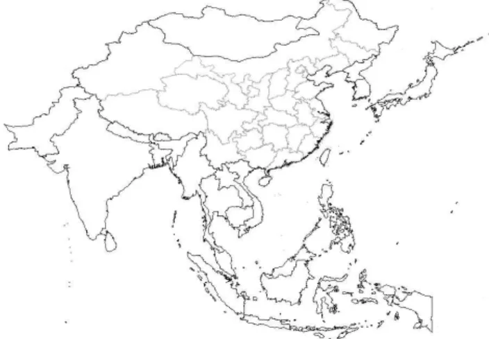
The key elements of the INTEX-B inventory are listed in Table 1. The domain covers 22 countries and regions in Asia and stretches from Pakistan in the West to Japan in the East and from Indonesia in the South to Mongolia in the North (Fig. 1). In this paper we emphasize emissions from China because they dominate the Asia pollutant outflow to the Pa-cific and the increase of emissions from China since 2000 is of great concern.
Emissions are estimated for eight major chemical species: SO2, NOx, CO, nonmethane volatile organic compounds (NMVOC), particulate matter with diameters less than or equal to 10µm (PM10), particulate matter with diame-ters less than or equal to 2.5µm (PM2.5), black carbon
aerosol (BC), and organic carbon aerosol (OC). Emissions of methane (CH4) and ammonia (NH3) were not updated from TRACE-P in this work, because they have not changed much since 2000, as confirmed by the REAS inventory (Ohara et al., 2007). In addition, CH4 and NH3 were low priori-ties of the INTEX-B mission (Singh et al., 2006). NMVOC emissions are speciated into five categories corresponding to five different chemical mechanisms (CBIV, CB05, RADM2,
Fig. 1.Definition of the inventory domain.
SAPRC99, and SAPRC07); this aspect of the inventory is described in a separate paper (Zhang et al., 2009).
Only anthropogenic emissions are estimated in this work. Biomass burning emissions were included in the TRACE-P inventory, but since then a number of new high-resolution biomass burning inventories have been developed using satellite observations of burning (e.g., Duncan et al., 2003; van der Werf et al., 2006; Randerson et al., 2007) that of-fer superior representation of emissions for specific years. TRACE-P biomass burning emissions can still be used by modelers interested in obtaining a typical representation of Asian biomass burning. The detailed emission calculations for the 2006 INTEX-B inventory are aggregated into four source categories: electricity generation, industry, residen-tial, and transportation.
Emission estimates in this work are specifically for the year 2006, because this inventory was prepared for the INTEX-B field campaign undertaken in spring 2006, and it was intended to reflect the actual magnitude of emissions during that period as closely as possible. However, when construction of the inventory took place in 2006 and 2007, most of the necessary statistics for Asian countries were only available for 2004/2005 and very few for the year 2006. Thus this inventory is built on a mixture of trend extrapolations from 2004/2005 and actual 2006 data.
Section 2 documents the methodology used in this work. The estimation of emissions from such a wide variety of species and regions cannot be described in complete de-tail due to space limitations. However, we give a general overview of methods, data, and data sources for this in-ventory and highlight the major advances from the previous TRACE-P inventory.
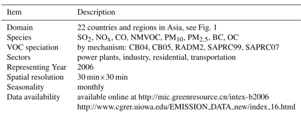
Table 1.Summary of the INTEX-B Asia emission inventory dataset.
Item Description
Domain 22 countries and regions in Asia, see Fig. 1
Species SO2, NOx, CO, NMVOC, PM10, PM2.5, BC, OC
VOC speciation by mechanism: CB04, CB05, RADM2, SAPRC99, SAPRC07
Sectors power plants, industry, residential, transportation
Representing Year 2006
Spatial resolution 30 min×30 min
Seasonality monthly
Data availability available online at http://mic.greenresource.cn/intex-b2006
http://www.cgrer.uiowa.edu/EMISSION DATA new/index 16.html
representation of actual emissions. In Sect. 3.1, we revisit China’s emissions for 2001 (R01), the year of the TRACE-P campaign, using our new methodology. Then the differences between R01 and T00 reflect the improvements and correc-tions made to the T00 inventory, and the changes between I06 and R01 represent actual growth in emissions in China between 2001 and 2006. Asian emission estimates by coun-try are presented in Sect. 3.2.
Emissions are initially calculated by country (by province for China) on an annual basis. However, emissions from some species have strong seasonal variations associated with such activities as fossil-fuel and biofuel use for home heat-ing in winter. The seasonality in emissions is important when comparing emissions with time-specific field measure-ments. For this reason, we have also developed monthly emissions using a variety of methods, which are discussed in Sect. 3.3. Atmospheric models also require gridded emis-sions as inputs, rather than regional emission totals. Sec-tion 3.4 presents the spatial distribuSec-tion of emissions at a res-olution of 30 min×30 min, using various spatial surrogates. All regional summaries and gridded data can be downloaded from several websites, as described in Sect. 3.5.
In the discussion section (Sect. 4), we compare our es-timates with other inventory studies. Top-down constraints on emissions also provide valuable clues for verifying emis-sion estimates, which have been successfully used in the re-vision and improvement of China’s CO emission inventory after the TRACE-P campaign (Streets et al., 2006). There-fore, in Sect. 4 we also compare our inventory with various top-down constraints, e.g., forward modeling, inverse mod-eling, and constraints from satellite and in-situ observations, and try to explain any discrepancies between inventories and top-down studies. In Sect. 4.3, we discuss the major uncer-tainties in this inventory and the future efforts that are needed to develop an even better understanding of Asian emissions. Finally, in Sect. 4.4, we summarize the relevant studies that have used this inventory and the implications for the present inventory.
2 Methodology
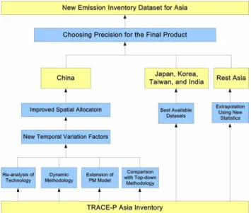
Figure 2 shows the general methodology for this inventory. We assemble the new Asian emission inventory according to the following steps. First, we implement a series of im-proved, technology-based methodologies to develop a new emission inventory for China. The key aspects of these im-provements are documented in Sect. 2.1. This same approach was used for the development of the improved CO inventory (Streets et al., 2006), the first primary particulate emission in-ventory (Zhang et al., 2006, 2007a), and a new NOxemission trend for China (Zhang et al., 2007b). We update China’s emissions to the year 2006 with these new methodologies. Second, we update emissions for other Asian countries to the year 2006 following the methodology of the TRACE-P inventory but using the most recent statistics available. Third, we incorporate the best available datasets for some selected regions, where good national inventories exist that are thought to be more accurate than the TRACE-P inven-tory, being built on local data sources and local knowledge. In this respect we have incorporated the following external data sources into the INTEX-B inventory: SO2and aerosol inventories for India (Reddy and Venkataraman, 2002a, b); a 1 km×1 km high-resolution emission inventory for Japan (Kannari et al., 2007); a South Korean inventory from the Na-tional Institute of Environmental Research of Korea (NIER, 2005, 2008), and a Taiwan inventory from the Taiwan Envi-ronmental Protection Administration (Fu et al., 2009). These override the TRACE-P updates. Finally, we check for con-sistency among the different datasets, choose the appropriate precision for the final product, and finally export the dataset over the whole of Asia with a uniform data format.
Fig. 2.Schematic methodology for the development of the INTEX-B Asia emission inventory.
The emissions of a particular species are estimated by the following equation:
Ei = X
j X
k Ai,j,k
" X
m
Xi,j,k,mEFj,k,m #
(1)
For a given technology m, the net emission factor is esti-mated as follows:
EF =EFRAW
X
n
Cn(1−ηn) (2)
whereirepresents the province (municipality, autonomous region); j represents the economic sector; k represents the fuel or product type; mrepresents the technology type for combustion and industrial process; n represents a specific control technology; A represents the activity rate, such as fuel consumption or material production; X is the fraction of fuel or production for a sector that is consumed by a spe-cific technology;EFis the net emission factor;EFRAWis the unabated emission factor; Cn is the penetration of control
technology n; and ηn, is the removal efficiency of control
technologyn.
2.1 Revision and improvement of the TRACE-P inventory for China
In this work, we have researched many aspects of the China part of the TRACE-P inventory for possible improvements by critical retrospective examination of how the original in-ventory was constructed and how well it performed in the various modeling and assessment projects in which it was used. We note the following major improvements thought to be necessary:
a) A detailed technology-based approach. The final re-lease rates of pollutants greatly depend on combustion effi-ciency, control equipment, and operating conditions. Thus, a detailed source classification by technology level is critical for obtaining reliable emission estimates. In the TRACE-P inventory, emitting sources were usually classified at the eco-nomic sector level, say, power generation, industry, or resi-dential, and an average emission factor was applied for the whole sector. However, in a rapidly developing country like China, both advanced and old-fashioned technologies co-exist in the marketplace, which can have very different levels of emissions. For example, the CO emission factors of indus-trial combustion devices can vary from 2 g/kg for large, mod-ern coal-fired boilers to 156 g/kg for old kilns, leading to an average emission factor of 85.7 g/kg for the industrial com-bustion sector as a whole, more than a factor of two greater than the value used in the TRACE-P estimates. We have suc-cessfully applied such a technology-based methodology to improve the CO emission inventory for China (Streets et al., 2006), and we expand the method to all species in this work. b) Re-examination of energy statistics. Data inconsis-tency in Chinese energy statistics downgrades the accuracy of emission inventories that largely rely on statistics (Aki-moto et al., 2006). In recent work on China’s NOx emis-sion trend (Zhang et al., 2007b), we critically evaluated the quality and reliability of current Chinese energy statistics and used several approaches for better representation of the real-world situation in China when compiling activity data. These approaches include: using coal consumption data in the provincial energy balance tables of the China Energy Statistical Yearbooks (CESY) to reflect the actual coal pro-duction and consumption; using diesel consumption data in the national energy balance table of CESY to avoid the “lost diesel” from inter-province transportation; and a model ap-proach for fuel consumption for each vehicle type, as these data are not available in statistics. We followed these proce-dures in this work. For more details, the reader is referred to Sects. 3.2, 3.3, and 4.5 of Zhang et al. (2007b).
d) A size-fractioned primary PM emission inventory. The emissions of two aerosol species, BC and OC, were esti-mated in the TRACE-P inventory, but primary PM10 and PM2.5emissions were not reported. In this paper, we present a comprehensive estimation of primary particulate emissions in China by size distribution and major components, using a technology-based approach described in Zhang et al. (2006, 2007a). With this approach, we are able to classify particu-late emissions into three size ranges, total suspended partic-ulates (TSP), PM10, and PM2.5(the latter two are reported in this paper), and also identify the contributions of BC and OC.
e) A new scheme of NMVOC speciation for model-ready emissions. NMVOCs differ significantly in their effects on ozone formation, and these differences need to be repre-sented appropriately in the air quality models used to predict the effects of changes of emissions on formation of ozone. This requires appropriate methods to specify the chemical composition of the many types of NMVOCs that are emit-ted and appropriate methods to represent these compounds in the models. In the TRACE-P inventory, NMVOC emis-sions were speciated into 19 categories based on chemical reactivity and functional groups. However, these emissions are usually not ready for model use: atmospheric modelers have to map those 19 categories into the categories that their models use. This conversion process is not accurate and can introduce unpredictable uncertainties.
In this work, we improve the NMVOC speciation method-ology toward an atmospheric-model-ready dataset by using a step-by-step VOC speciation assignment process. Emis-sions for individual VOC species are calculated by apply-ing a state-of-the-art source profile database (e.g., Liu et al., 2008) to each source category. Then we lump indi-vidual NMVOC emissions to emitted species in different chemistry mechanisms. Up to now, we have developed model-ready emissions for five mechanisms: CBIV, CB05, RADM2, SAPRC99, and SAPRC07. The detailed descrip-tion of this methodology and the results are presented in a separate paper (Zhang et al., 2009).
f) Comparison with top-down constraints. Last, but not least, top-down analytical tools applied to the interpretation of emissions provide valuable constraints to improve bottom-up emission inventories such as this one. Such techniques include forward modeling and inverse modeling using in situ and satellite observations, or even simply using observation data without models. In the years after the TRACE-P mis-sion, these techniques have become widely used to constrain Asian emissions against a priori estimates. The results of these analyses sometimes support the inventory, while more often they raise questions about the accuracy of the inventory. In Sects. 4.1 and 4.2 of this paper, we present an intensive review of these analyses, discuss the existing discrepancies, and attempt to find a direction to reconcile the inventory in light of these findings.
2.2 Activity rates 2.2.1 China
We derive activity data for China for the years 2001 and 2006 from a wide variety of sources, with a critical examination of the data reliability. Fuel consumption in stationary combus-tion sources by sector and by province (Ain Eq. 1) is de-rived from the provincial energy balance tables of the CESY (National Bureau of Statistics, 2004, 2007a), with the ex-ception of diesel consumption. We use diesel consumption values in the national energy table of CESY and then derive shares from the provincial tables (see explanation in item
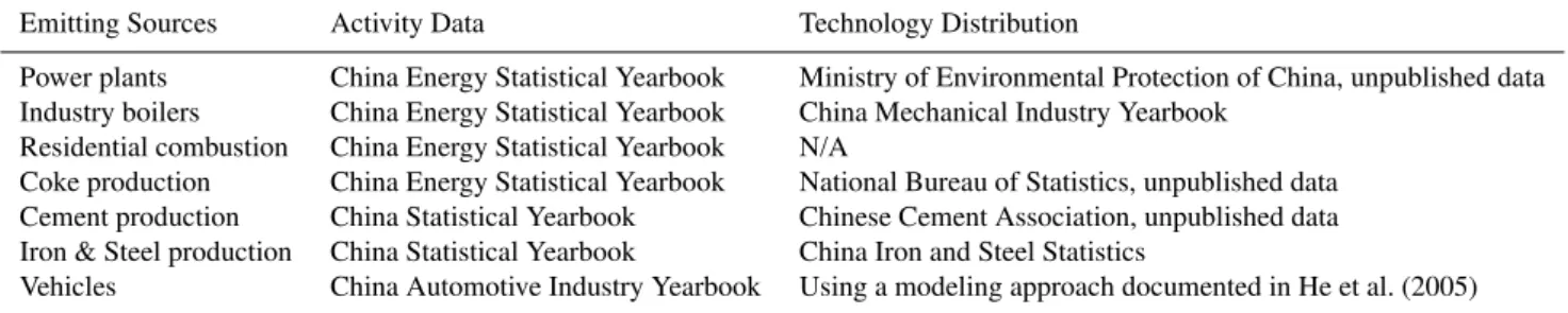
b of Sect. 2.1). Industrial production by products and by province is derived from other governmental statistics (Na-tional Bureau of Statistics, 2002a, b, 2006, 2007b; AISIC, 2002, 2006). The methods for determining activity levels of non-energy sources for NMVOC are the same as in pre-vious analyses (Klimont et al., 2002). The distributions of the combustion technology in each sector and the processing technology in each industrial product (X in Eq. 1) are gen-erally not available from government statistics. In this work, these data were collected from a wide range of unpublished statistics by various industrial association and technology re-ports. The data sources of key emitting sources in China are summarized in Table 2.
When this inventory was developed in 2006 and 2007, most of the available statistics for Chinese provinces were for 2004/2005 and very few for the year 2006. We there-fore extrapolated activity data to the year 2006 based on var-ious fast-track statistics that are published monthly (Beijing Huatong Market Information Co. Ltd., various issues, 2006; China Statistical Information and Consultancy Center, vari-ous issues, 2006).
We classify vehicles into light-duty gasoline vehicles (LDGV), light-duty gasoline trucks up to 6000 lb gross ve-hicle weight (LDGT1), light-duty gasoline trucks with gross vehicle weight 6001–8500 lb (LDGT2), light-duty diesel trucks (LDDT), heavy-duty gasoline vehicles (HDGV), heavy-duty diesel vehicles (HDDV), and motorcycles, corre-sponding to the classification method in the US EPA’s MO-BILE emission factor model. It is not possible to derive the fuel consumption for each vehicle type from CESY. As an al-ternative approach we estimate fuel consumption from vehi-cle population, annual average vehivehi-cle mileage traveled, and fuel economy for each vehicle type. This method has been documented in our previous work (Streets et al., 2006), and the full details of the model used and the methodological ap-proach are described elsewhere (He et al., 2005).
2.2.2 Other Asian countries
Table 2.The data sources of key emitting sources in China.
Emitting Sources Activity Data Technology Distribution
Power plants China Energy Statistical Yearbook Ministry of Environmental Protection of China, unpublished data
Industry boilers China Energy Statistical Yearbook China Mechanical Industry Yearbook
Residential combustion China Energy Statistical Yearbook N/A
Coke production China Energy Statistical Yearbook National Bureau of Statistics, unpublished data
Cement production China Statistical Yearbook Chinese Cement Association, unpublished data
Iron & Steel production China Statistical Yearbook China Iron and Steel Statistics
Vehicles China Automotive Industry Yearbook Using a modeling approach documented in He et al. (2005)
use by fuel type, sector, and country instead of the RAINS-ASIA database. Activity data for the year 2006 are ex-trapolated from 2000–2004 IEA energy data using the av-erage growth rate during 2000–2004. Technology distribu-tions within each sector were obtained from the IMAGE 2.2 database (RIVM, 2001). Industrial production by product and country is derived from United States Geological Sur-vey statistics (USGS, 2006) and also extrapolated to the year 2006. The methods for determining activity levels of non-energy sources of NMVOC are the same as in previous work (Klimont et al., 2001).
2.3 Emission factors
Emission factors for the years 2001 and 2006 for China are developed using our dynamic, technology-based methodol-ogy. We assume that the emission rate is fixed over the years for a given combustion/process technology (min Eq. 1) and control technology (nin Eq. 2). Development of emission factors by technology has been documented in our previous work (Klimont et al., 2002; Streets et al., 2006; Zhang et al., 2006, 2007a, b). However, for a fast developing coun-try like China, new technologies are constantly coming into the marketplace, causing rapid changes in the penetration of technologies (Xin Eq. 1 andCnin Eq. 2) and therefore rapid
changes in net emission factors for a fuel/product in a spe-cific sector. We estimate year-by-year changes inXandCn,
where possible.
In some cases, we use the same emission factors for the years 2001 and 2006. For example, VOC emission factors of various industrial processes are the same for the years 2001 and 2006, because we are not aware of any VOC capture technologies being used for those processes. We also use fixed emission factors for many small combustion devices like coal and biofuel stoves because there is no efficient way to control their emissions. But for most sectors, net emission factors were fundamentally changed to reflect the dramatic economic growth and dynamic technology penetration. Ta-ble 3 summarizes the significant changes of emission factors between 2006 and 2001 in China.
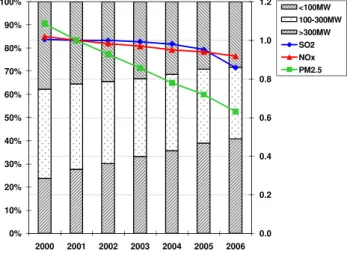
Environmental legislation is always an important determi-nant of emission factors. For example, the Chinese govern-ment has announced an ambitious plan to reduce national SO2 emissions by 10% in 2010 compared with 2005. To achieve this goal, flue-gas desulfurization (FGD) devices are now being widely installed in coal-fired power plants. From 2001 to 2006, FGD penetration increased from 3% to 30%, causing a 15% decrease in the average SO2emission factor for coal-fired power plants (see Fig. 3a). Likewise, during the same period, net PM2.5emission factors in power plants declined from 2.0 g/kg coal to 1.2 g/kg coal, a reduction of 40%. This reduction is largely attributed to a new, strength-ened PM emission standard for power plants published in 2003 (SEPA, 2003).
A series of emission standards was implemented for new vehicles in 1999, as shown in Table 4. Since then, new ve-hicles with advanced emission-control technologies began to join the fleet and replace old ones. In 2006, 60% of on-road gasoline vehicles could meet EURO II or EURO III emis-sion standards, increased from 1% in 2001. As a result, from 2001 to 2006, the average emission factors of gasoline vehi-cles decreased by 23% for NOx, 54% for CO, and 36% for VOC (Fig. 3b).
0.0 0.2 0.4 0.6 0.8 1.0 1.2
0% 10% 20% 30% 40% 50% 60% 70% 80% 90% 100%
2000 2001 2002 2003 2004 2005 2006
<100MW 100-300MW >300MW SO2 NOx PM2.5
a) coal-fired power plants
0.0 0.2 0.4 0.6 0.8 1.0 1.2
0% 10% 20% 30% 40% 50% 60% 70% 80% 90% 100%
2000 2001 2002 2003 2004 2005 2006
Euro III Euro II Euro I Euro 0 NOx CO VOC
b) gasoline vehicles
Fig. 3.Technology renewal and average emission factors for China.
Bars represent the percentage of each technology: (a)share of
power units with different boiler size;(b)share of gasoline
vehi-cles with different stages of control technologies. Line: trends of average emission factors. All data are normalized to the year 2001.
unpublished data, 2007), leading to a 25% decrease in the average CO emission factor but a 35% increase in the aver-age NOxemission factor of China’s cement plants.
For other Asian countries, we have generally used the same emission factors as in the TRACE-P inventory. An ex-ception is for vehicle emissions. Emission factors for vehi-cles were derived using the MOBILE model, by integrating the varying stages of emission restrictions in recent years, to reflect the changes of emission factors due to implementation of emission standards.
3 Results
3.1 China emissions
3.1.1 Revisiting 2001 emissions: learning from methodology improvements
With the improved methodology described above, we es-timate China’s anthropogenic emissions in the year 2001 as follows: 22.9 Tg SO2, 13.4 Tg NOx, 141.6 Tg CO, 18.1 Tg NMVOC, 16.1 Tg PM10, 11.7 Tg PM2.5, 1.6 Tg BC,
and 2.8 Tg OC. Table 5 summarizes the 2001 emission esti-mates by species and by sector and presents the difference between this 2001 inventory (R01) and the TRACE-P inven-tory for the year 2000 (T00). R01 estimates generally show a significant increase compared with T00, ranging from a 6% increase for OC to 70% for BC. Because the actual emission increases from 2000 to 2001 were not so significant (e.g., 5% increase for NOx), these differences between R01 and T00 can be mainly attributed to the improvements of methodol-ogy.
The reasons for these differences vary among sectors and species. The most important reason is that R01 uses a technology-based approach that can identify emissions from specific types of technology. For example, industrial CO emissions in R01 are higher than in T00 by a factor of three, contributing significantly to the difference of CO emissions between T00 and R01. Compared with T00, R01 has a much more detailed categorization of sources in the industrial sec-tor, which allows the identification of important CO emit-ting sources from specific industries such as cement kilns and brick kilns, which were missing in T00 (Streets et al., 2006). The situation is similar for other species. In R01, traditional brick kilns and coking production are identified as two important individual sources for BC and OC emis-sions. Using emission factors from Bond et al. (2004), BC emissions from traditional brick kilns and coking processes for the year 2001 are estimated to be 241 Gg and 183 Gg, respectively, accounting for 15.1% and 11.5% of total an-thropogenic emissions. These two important carbonaceous aerosol sources were missing in T00.
Table 3.Changes of emission factors between 2006 and 2001.
Sector Fuel/product Species Unit Emission Factor Reason for Change
2006 2001
Power plants coal SO2 g/kg-coal 15.4 18.1 Installation of FGD required by government
coal NOx g/kg-coal 7.1 7.8 Increased market share of large units
coal PM2.5 g/kg-coal 1.2 2.0 Implementation of new emission standarda
Cement kilns coal/cement NOx g/kg-coal 8.1 6.0 Shift from shaft kilns to rotary kilns,
coal/cement CO g/kg-coal 90.4 121.0 which release less CO but more NOx
coal/cement PM2.5 g/kg-cement 3.3 6.5 Implementation of new emission standarda
Brick kilns coal/brick CO g/kg-coal 128.0 150.0 Phase out of old beehive kilns
coal/brick BC g/kg-coal 2.6 3.3
Coke production coke CO g/kg-coke 4.1 5.6 Phase out of old indigenous process
coke BC g/kg-coke 0.77 1.8
Iron & steel production sinter, pig ironb CO g/kg-iron 39.6 59.0 Increased ratio of by-pass gas recycle in
steel CO g/kg-steel 24.0 37.0 new factories
sinter, pig ironb PM2.5 g/kg-iron 0.55 0.85 New factories with lower emissions come
steel PM2.5 g/kg-steel 0.32 0.51 into the marketplace
Gasoline vehiclesc,d gasoline NOx g/kg-fuel 21.5 28.0 New emission standards were implemented
gasoline CO g/kg-fuel 294.2 633.3 in 1999; new vehicles rapidly replace
gasoline VOC g/kg-fuel 88.4 139.1 old vehicles
Diesel vehiclesc,e diesel NOx g/kg-fuel 55.2 65.0 Same as gasoline vehicles
diesel CO g/kg-fuel 59.1 116.1
diesel VOC g/kg-fuel 15.7 31.1
diesel PM2.5 g/kg-fuel 3.1 4.2
aSEPA (2003, 2004);b emission factors are given for the sum of sintering processes and pig iron production; cemission factors were
calculated by MOBILE model in g/km, then converted to g/kg-fuel according to the fleet average fuel economy data of He et al. (2005);
demission factors were calculated for LDGV (car), LDGT1, LDGT2, and HDGV separately. Here average emission factors are presented;
eemission factors were calculated for LDDT and HDDT separately. Here average emission factors are presented.
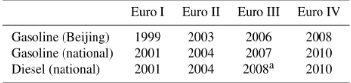
Table 4.Implementation schedule of new vehicle emission standards in China.
Euro I Euro II Euro III Euro IV
Gasoline (Beijing) 1999 2003 2006 2008
Gasoline (national) 2001 2004 2007 2010
Diesel (national) 2001 2004 2008a 2010
ainitially scheduled for 2007, but postponed to 2008.
Different data sources can also lead to different results. For the power plant sector, SO2and NOxemissions in R01 are both 22% higher than in T00. This is mainly because the coal consumption data used in R01 are actual statistical data from CESY, while the data used in T00 were extrapolated from 1995 data, which was lower than in the actual reported statistics. SO2emissions for transportation in R01 are 82% lower than in T00 because we use lower sulfur contents for
transportation fuels – though the contribution of the trans-portation sector to total SO2emissions is small.
3.1.2 2006 emissions: emission growth and driving forces
We estimate China’s anthropogenic emissions in the year 2006 to be as follows: 31.0 Tg SO2, 20.8 Tg NOx, 166.9 Tg CO, 23.2 Tg NMVOC, 18.2 Tg PM10, 13.3 Tg PM2.5, 1.8 Tg BC, and 3.2 Tg OC. Table 6 presents
the 2006 emission estimates and Fig. 4 shows the emission increase from 2001, by species and by sector. Compared with the decreasing or flat emission trend during 1995–2000 (Hao et al., 2002; Streets et al., 2001), all species show an increasing trend during 2001–2006: 36% increase for SO2, 55% for NOx, 18% for CO, 29% for VOC, 13% for PM10, and 14% for PM2.5, BC, and OC. These emission
Table 5.Anthropogenic emissions in China in the year 2001 (units: Gg/year).∗
Species Power Industry Residential Transportation Total
SO2 12 270 (1.22) 7946 (1.08) 2599 (1.03) 75 (0.18) 22 891 (1.13)
NOx 5390 (1.22) 3405 (1.22) 997 (1.42) 3604 (1.37) 13 397 (1.27)
CO 1861 (n/a) 53 526 (2.97) 48 254 (1.10) 37 930 (1.00) 141 571 (1.42)
NMVOC 547 (6.02) 4982 (1.34) 5996 (1.07) 6547 (1.23) 18 072 (1.23)
PM10 1873 (n/a) 9647 (n/a) 4258 (n/a) 292 (n/a) 16 070 (n/a)
PM2.5 1152 (n/a) 6398 (n/a) 3853 (n/a) 284 (n/a) 11 687 (n/a)
BC 38 (5.59) 545 (6.13) 868 (1.11) 143 (2.40) 1595 (1.70)
OC 8 (1.52) 496 (17.95) 2254 (0.88) 70 (1.35) 2827 (1.06)
∗Numbers in parentheses represent the emission ratio between this inventory for the year 2001 (R01) and the TRACE-P inventory for the
year 2000 (T00).
Table 6.Anthropogenic emissions in China in the year 2006 (units: Gg/year).∗
Species Power Industry Residential Transportation Total
SO2 18 333 (1.49) 9725 (1.22) 2838 (1.09) 123 (1.64) 31 020 (1.36)
NOx 9197 (1.71) 5371 (1.58) 1166 (1.17) 5096 (1.41) 20 830 (1.55)
CO 2362 (1.27) 74 936 (1.40) 55 883 (1.16) 33 709 (0.89) 166 889 (1.18)
NMVOC 961 (1.76) 8056 (1.62) 7601 (1.27) 6630 (1.01) 23 247 (1.29)
PM10 2476 (1.32) 10 436 (1.08) 4884 (1.15) 427 (1.46) 18 223 (1.13)
PM2.5 1474 (1.28) 6932 (1.08) 4461 (1.16) 398 (1.40) 13 266 (1.14)
BC 36 (0.94) 575 (1.06) 1002 (1.15) 198 (1.38) 1811 (1.14)
OC 6 (0.72) 505 (1.02) 2606 (1.16) 101 (1.45) 3217 (1.14)
∗Numbers in parentheses represent the emission ratio between the year 2006 (I06) and the year 2001 (R01).
It is quite clear that the dramatic emission increases in China after 2001 were driven by the economic boom and growing infrastructure investments. Figure 5 shows how China’s power plants grew during 2001–2006 compared with the previous five years. Many energy-consuming activities doubled in just a few years in China, resulting in a significant increase in relevant emissions. For example, total thermal based electricity generation increased from 1.17 trillion kWh in 2001 to 2.37 trillion kWh in 2006, and total vehicle num-bers increased from 18 million to 37 million during the same period.
On the other hand, China has made substantial efforts on technology improvement and emission control during this period. These measures have offset the emission growth sig-nificantly. We note several developments that have had im-portant impacts on emissions in the following areas:
a) New technologies with improved energy intensity and/or lower emissions.These technologies include: replacement of small power generation boilers by large ones that have better combustion efficiencies; use of power generation boilers with LNB technologies to reduce NOxemissions; replacement of indigenous processes by modern processes for coke produc-tion, resulting in a significant reduction of emissions; transi-tion from shaft kilns to new-dry kilns in the cement industry, which reduces CO emissions (but increases NOxemissions);
-1 0 1 2 3 4 5 6 7 8 9
SO2 NOx CO/10 NMVOC PM10 PM2.5 BC*10 OC*10
C
h
a
n
g
e
of
Em
is
s
ion
s
(
T
g)
Transportation Residential Industry Power
Fig. 5. NOx emission increase from China’s power plants. Left
panel: NOxemission change from China’s power plants between
2001 and 1996. Right panel: NOxemission change from China’s
power plants between 2006 and 2001 (units: Mg per grid).
and advanced technologies to capture by-pass gas during iron and steel production, to avoid the CO releases from by-pass gas.
b) FGD installation on coal-fired power plants. As dis-cussed in Sect. 2.3, FGD has been widely installed in power plants in recent years under new requirements of central and local government. By the end of 2006, 30% of coal-fired power plants were equipped with FGD, which is estimated to eliminate about 6 Tg of SO2emissions in that year. FGD penetration in power plants further increased to 50% at the end of 2007, leading to a 4.7% reduction of national SO2 emissions in 2007, which is the first decrease in national SO2 emissions since the year 2002 (MEP, 2008).
c) Strengthened PM emission standards for cement plants and coal-fired power plants. Cement plants and coal-fired power plants contributed 37% and 10% of national PM2.5 emissions, respectively in 2001. In 2003 and 2004, China implemented new emission standards for these two sectors, which strengthened the limits for TSP emissions from 150– 600 mg/Nm3 to 50–100 mg/Nm3for all cement plants, and from 200–600 mg/Nm3 to 50 mg/Nm3 for new coal-fired power plants (SEPA, 2003, 2004; CRAES, 2003). To meet these standards, high-efficiency PM removal equipment was widely installed, and some small, dirty factories were closed. As a result, PM2.5emissions from cement plants and coal-fired power plants decreased by 7% and increased by 23% during 2001–2006, respectively, in contrast to the doubled activity rates in each sector.
d) Emission standards for new vehicles. Table 4 lists the emission standards for new vehicles in China in recent years, and Fig. 3b shows the decreasing trend of emission factors when new vehicles join the fleet and replace old ones. CO emissions from the transportation sector decreased by 11% during 2001–2006 during a period when the total number of vehicles doubled, providing an excellent illustration of effec-tive control measures. NMVOC emissions in 2006 were
al-most the same as in 2001, while NOxemissions increased by 41%, but still showing a much lower growth than the growth in the vehicle population.
Table 7 presents China’s emissions by province for the year 2006. Emissions vary considerably from province to province, with the highest emissions mainly located in the eastern and central regions of China. Hebei, Henan, Jiangsu, Shandong, and Sichuan Provinces are the five largest contrib-utors for most species. Shandong is the largest contributor for SO2, NOx, NMVOC, PM10, and PM2.5 and the second largest contributor for CO and OC. Emissions from western provinces, e.g., Qinghai and Xizang, were much less than from eastern ones. The regional differences of emissions are mainly caused by differences of economic development, in-dustry structure, and population.
3.2 Total Asian emissions
We estimate total Asian anthropogenic emissions in the year 2006 as follows: 47.0 Tg SO2, 36.8 Tg NOx, 298.1 Tg CO, 54.6 Tg NMVOC, 28.9 Tg PM10, 22.0 Tg PM2.5, 2.91 Tg BC,
and 6.54 Tg OC. These values are not directly comparable with the TRACE-P inventory due to the fundamental changes in methodologies discussed previously. However, most im-pacts of methodology improvement can be removed by re-placing the China part of the TRACE-P inventory with the R01 inventory of this work. Then we can compare the re-vised TRACE-P Asian emissions with our new estimates, to explore the actual emission changes during the interven-ing years. Asian emissions continue the significant increas-ing trends that have been reported in the last two decades (van Aardenne et al., 1999; Streets et al., 2001; Ohara et al., 2007). From the beginning of the 21st century, Asian anthro-pogenic emissions increased by 33% for SO2, 44% for NOx, 18% for CO, 25% for NMVOC, and 9% for BC in just 5 years. The most significant growth was found for NOx sions, which is driven by both industrial and vehicular emis-sions. In contrast, BC emissions, which are dominated by the residential sector, show a relatively small increase. OC emis-sions decreased by 9%, but this cannot be viewed as a real emission decrease, because in this 2006 inventory we used lower estimates of emissions from Reddy and Venkatara-man (2002a, b) than the TRACE-P estimates. Reddy and Venkataraman (2002a, b) estimated that the OC emissions in India were 1.0 Tg in 1999, much lower than TRACE-P estimates of 2.2 Tg in 2000. The main reason for this dif-ference is that Reddy and Venkataraman (2002b) used lower OC emission factors for biofuel combustion.
Table 7.Anthropogenic emissions in China by province in 2006 (units: Gg/year).
Province SO2 NOx CO VOC PM10 PM2.5 BC OC
Anhui 693 715 7986 958 757 574 84 173
Beijing 248 327 2591 497 123 90 19 19
Chongqing 1211 326 2928 343 340 257 34 75
Fujian 460 547 3895 701 435 337 44 127
Gansu 338 323 2688 303 296 222 35 55
Guangdong 1175 1493 8693 1780 942 680 55 120
Guangxi 880 435 4258 640 468 348 40 94
Guizhou 1952 485 4409 481 571 435 90 162
Hainan 76 83 724 117 67 53 7 18
Hebei 2281 1308 15 505 1521 1371 981 137 200
Heilongjiang 242 839 4967 771 579 440 72 144
Henan 1591 1197 10 957 1289 1193 834 133 197
Hong Kong 118 148 127 109 27 18 1 1
Hubei 2200 930 7482 875 772 559 73 137
Hunan 915 563 5124 641 576 424 54 105
Jiangsu 1697 1486 11 326 1814 1200 881 87 186
Jiangxi 533 390 3963 463 586 400 39 76
Jilin 357 473 3794 523 395 293 45 82
Liaoning 1027 955 8105 989 710 512 64 111
Nei Mongol 1171 860 5253 575 574 420 71 113
Ningxia 380 175 961 131 134 98 11 18
Qinghai 18 46 616 74 70 54 8 11
Shaanxi 907 352 3528 491 474 328 49 81
Shandong 3102 1759 14 970 2093 1702 1212 132 213
Shanghai 618 631 1958 594 138 91 10 8
Shanxi 1804 934 5787 627 969 669 139 158
Sichuan 2555 873 10 945 1312 1068 845 133 318
Tianjin 336 365 1860 381 161 109 15 18
Xinjiang 210 356 2775 391 257 194 37 55
Xizang 0 5 94 14 9 6 1 1
Yunnan 489 344 3765 515 454 343 56 97
Zhejiang 1434 1106 4857 1233 806 556 36 45
China Total 31 020 20 830 166 889 23 247 18 223 13 266 1811 3217
OC. India follows China as the second largest contributor with the following shares: 12% for SO2, 13% for NOx, 20% for CO, 20% for NMVOC, 14% for PM10, 14% for PM2.5, 12% for BC, and 14% for OC. Other countries
con-tribute much smaller individual shares. China’s contribution to Asian emissions has increased since the year 2000, reflect-ing faster economic development and industrialization than other Asian developing countries. South Asia and Southeast Asia contribute significantly to emissions of CO, NMVOC, and OC, due to the large amount of residential biofuel use.
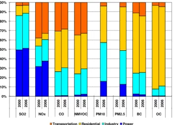
Figure 7 compares the sectoral contributions of Asian emissions in 2000 and 2006. The sectoral distribution of emissions is similar between the two years, with some small but meaningful changes. The contribution from power plants to SO2and NOx emissions has increased, driven by the in-dustrialization progress and spread of electrification in the past years. Although the vehicle stocks in Asia increased
0 50 100 150 200 250 300 350
0% 10% 20% 30% 40% 50% 60% 70% 80% 90% 100%
SO2 NOx CO NMVOC PM10 PM2.5 BC OC
E
m
issi
ons
(
T
g)
Pe
rc
e
n
t
Other South Asia India Southeast Asia Other East Asia
China Total
Table 8.Summary of national emissions in Asia in 2006 (units: Gg/year).
Country SO2 NOx CO NMVOC PM10 PM2.5 BC OC
China 31 020 20 830 166 889 23 247 18 223 13 266 1811 3217
Japana 871 2404 5314 2033 195 141 51 21
Korea, Rep of 408b 1307b 789b 796b 67b 54 17 11
Korea, DPR 233 270 3583 212 301 245 21 95
Mongolia 84 38 351 23 27 22 2 9
Taiwan, Chinac 189 642 1672 864 337 175 91 9
Brunei 7 23 15 46 4 3 0 0
Cambodia 34 27 570 113 68 61 7 32
Indonesia 1451 1583 17 742 6617 1838 1610 170 803
Laos 8 18 195 61 22 20 2 11
Malaysia 1137 1664 4286 1267 471 322 14 40
Myanmar 51 85 2568 641 271 244 29 130
Philippines 943 310 1998 1157 231 199 23 96
Singapore 163 193 149 101 32 22 2 1
Thailand 1299 1278 7189 2638 475 388 49 141
Vietnam 385 330 9843 1441 737 657 90 326
Bangladesh 148 182 3218 550 438 390 43 205
Bhutan 5 5 97 21 12 11 1 6
India 5596d 4861 61 106 10 767 4002 3111 344d 888d
Nepal 31 27 1659 251 205 186 21 103
Pakistan 2882 681 7378 1405 873 752 115 349
Sri Lanka 98 72 1501 371 100 88 11 44
Asia 2006 Total 47 045 36 829 298 112 54 620 28 930 21 967 2914 6537
Asia 2000 Totale 35 450 25 540 252 891 43 538 n/a n/a 2679 7209
2006/2000 1.33 1.44 1.18 1.25 n/a n/a 1.09 0.91
aFrom Kannari et al. (2007);bfrom NIER (2008);cfrom Fu et al. (2009);dbased on Reddy and Venkataraman (2002a, b) and scaled to
the year 2006;ehere Asia 2000 emissions consist of R01 inventory for China and TRACE-P inventory for other Asian countries, to better
represent the real-world Asia emissions around the year 2000.
0% 10% 20% 30% 40% 50% 60% 70% 80% 90% 100%
2000 2006 2000 2006 2000 2006 2000 2006 2000 2006 2000 2006 2000 2006 2000 2006
SO2 NOx CO NMVOC PM10 PM2.5 BC OC
Transportation Residential Industry Power
Fig. 7.Share of emissions by sector in Asia in 2000 and 2006.
dramatically during the past few years, the relative contri-butions from the transportation sector decreased for NOx, CO, and NMVOC, indicating the effectiveness of control measures on gasoline vehicles. However, the increasing contribution of transportation emissions to carbonaceous aerosols indicates the expanding diesel vehicle fleet and slow progress on control measures for diesel particles.
3.3 Seasonality of emissions
Table 9.Monthly anthropogenic emissions in China in 2006 (units: Gg/month).
Species Jan Feb Mar Apr May Jun Jul Aug Sep Oct Nov Dec
SO2 2853 2416 2628 2368 2389 2430 2472 2485 2460 2503 2794 3220
NOx 1839 1666 1770 1627 1631 1654 1667 1675 1667 1697 1866 2071
CO 18 051 15 123 14 677 12 194 12 131 12 382 11 714 11 911 12 302 12 806 15 041 18 552
NMVOC 2528 2154 2034 1707 1702 1727 1663 1684 1720 1778 2037 2513
PM10 1808 1516 1575 1356 1361 1401 1320 1346 1395 1445 1673 2026
PM2.5 1416 1166 1163 963 962 986 934 951 982 1023 1211 1507
BC 240 189 168 120 117 118 114 116 118 126 164 221
OC 511 385 310 193 185 183 182 183 182 200 283 419
Fig. 8.Emission distributions at 30 min×30 min resolution of gaseous species (units: Mg/year per grid).
Table 9 presents monthly emissions in China in 2006 by species. Strong seasonal variations are observed for CO, BC, and OC, where the residential sector contributes the largest portion of emissions. The ratios of monthly CO, BC, and OC emissions between maxima and minima are 1.6, 2.1, and 2.8, respectively. In contrast, SO2and NOxemissions have weaker seasonal variations, with ratios of 1.4 and 1.3 be-tween maxima and minima, because they mainly come from industrial and transportation emissions that have less of a sea-sonal cycle. We also find that SO2 and NOx emissions in
February are lower than in neighboring months, because of reduced industrial activity during the Chinese Spring Festival holiday.
3.4 Gridded emissions
Fig. 9.Emission distributions at 30 min×30 min resolution of aerosol species (units: Mg/year per grid).
and India, where the emissions were obtained from na-tional inventories, we keep the spatial distribution character-istics of the original inventories and simply re-grid them to 30 min×30 min resolution. All power generation units with capacity larger than 300 MW (∼400 units) in China are iden-tified as large point sources, while other plants are treated as area sources.
3.5 Data access
All regional and gridded emission data sets can be down-loaded from our web site (http://mic.greenresource.cn/ intex-b2006). Users can examine emissions by country and by sector from the summary tables. Gridded data include the emissions of all species by sector (power, industry, res-idential, and transportation) at 30 min×30 min resolution. At the time this paper was submitted, NMVOC emissions speciated according to the SAPRC-99 mechanism are avail-able by sector (power, industry, residential biofuel, residen-tial fossil fuel, residenresiden-tial non-combustion, and transporta-tion) for download at 30 min×30 min resolution, but we will add speciated VOC emissions for other mechanisms later. These emission data are also downloadable from the web-site at the University of Iowa (http://www.cgrer.uiowa.edu/ EMISSION DATA new/index 16.html).
4 Discussion
4.1 Magnitude of China’s emissions in inventories and top-down constraints
Ohara et al. (2007) conducted a comprehensive comparison of different emission inventories for Asia, China, and India during 1995–2000 and discussed the reasons for the differ-ences. In this section, we will not repeat that comparison, but focus instead on a comparison of the magnitude of China’s emissions in inventories and from top-down constraints for years after 2000 (Table 10), in order to highlight the implica-tions for emission inventory development.
Table 10.Estimates of China’s and East Asian annual emissions after the year 2000.a
Pollutant and Study Methodb Sourcesc Region 2000 2001 2002 2003 2004 2005 2006 SO2
Streets et al. (2003a) EI FF+BF China 20.3 Olivier et al. (2005) EI FF+BF China 34.2
Ohara et al. (2007) EI FF+BF China 27.6 29.3 31.9 36.6
SEPA EI FFd China 20.0 19.5 19.3 21.6 22.5 25.5 25.9
This work EI FF+BF China 22.9 31.0
NOx
Streets et al. (2003a) EI FF+BF China 10.5 Olivier et al. (2005) EI FF+BF China 13.7
Ohara et al. (2007) EI FF+BF China 11.2 11.8 12.7 14.5
Zhang et al. (2007b) EI FF+BF China 12.6 13.2 14.4 16.2 18.6 19.8 20.8
and this work
Wang et al. (2004) IM FF+BF+BB+SL China 16.5
Jaegle et al. (2005) IM FF+BF China 14.5
Martin et al. (2006) IM FF+BF+BB+SL East Asia 32.2
CO
Streets et al. (2003a) EI FF+BF China 100 Olivier et al. (2005) EI FF+BF China 87
Streets et al. (2006) EI FF+BF China 142 167
and this work
Ohara et al. (2007) EI FF+BF China 137 141 146 158
Palmer et al. (2003a) IM FF+BF China 168
Arellano et al. (2004) IM FF+BF+BB East Asia 196–214 Heald et al. (2004) IM FF+BF+BB East Asia 192
Wang et al. (2004) IM FF+BF+BB China 166
Petron et al. (2004) IM FF+BF+BB East Asia 186
Yumimoto and Uno (2006) IM FF+BF+BB China 147
Tanimoto et al. (2008) IM FF+BF+BB China 170
Kopacz et al. (2009) IM FF+BF+BB China 141.5
Carmichael et al. (2003b) FM FF+BF+BB China 163–210
Heald et al. (2003) FM FF+BF+BB China 181
Allen et al. (2004) FM FF+BF China 145
Tan et al. (2004) FM FF+BF+BB China 174
VOC
Streets et al. (2003a) EI FF+BF China 14.7 Olivier et al. (2005) EI FF+BF China 11.5
Wei et al. (2008) EI FF+BF China 20.1
Bo et al. (2008) EI FF+BF+BB China 11.0 16.5
This work EI FF+BF China 18.1 23.2
Fu et al. (2007) IM FF+BF+BB China 21.7e BC/OC
Streets et al. (2003a) EI FF+BF China 0.94/2.66 Bond et al. (2004) EI FF+BF China 1.36/2.11 Cao et al. (2006) EI FF+BF China 1.40/3.81
Ohara et al. (2007) EI FF+BF China 1.09/2.56 1.10/2.58 1.11/2.60 1.14/2.62
This work EI FF+BF China 1.60/2.83 1.81/3.22
aUnits are Tg/year. Units for NO
xare Tg-NO2/year.bEI = emission inventory; IM = inverse modeling; FM = forward modeling.cFF = fossil
fuel; BF = biofuel combustion; BB = open biomass burning; and SL = soil emissions.dOnly includes fossil-fuel emissions from power plants
and industry.eFu et al. (2007), required a 25% increase in reactive VOC emissions from the TRACE-P inventory (including BB emissions)
to agree with inverse modeling.
values estimated by REAS (Ohara et al., 2007) and EDGAR (Olivier et al., 2005).
It appears that the magnitude of China’s SO2 emissions in the TRACE-P inventory is reasonable on the basis of CTM model simulations and comparison with in situ mea-surements (Carmichael et al., 2003b; Russo et al., 2003; Tan
surface emissions (Richter et al., 2006; Krotkov et al., 2008). Further trend analysis of satellite SO2columns over China may be able to provide valuable information for verifying SO2emissions.
b) Nitrogen Oxides.NOxemission estimates for China are all quite close (see Table 10). Analysis from modeling and measurements during the TRACE-P campaign also indicated that the estimates of China’s NOxemissions in the TRACE-P inventory are reasonably accurate (Carmichael et al., 2003b). However, several inverse modeling analyses constrained by satellite-based data concluded that China’s NOx emission inventory was significantly underestimated (Martin et al., 2003, 2006; Jaegl´e et al., 2005; Wang et al., 2007). In the meantime, forward modeling studies also under-predicted NO2columns compared to satellite retrievals by a factor of two over East China, which is usually attributed to under-estimation of NOx emissions (Ma et al., 2006; Uno et al., 2007). China’s NOx emissions are mainly contributed by power plants and vehicles, and there is no clear evidence to suggest such a remarkable underestimation of emissions from those two sectors from the perspective of inventory de-velopment. One plausible reason is that current estimates of soil NOxemissions are too low (Wang et al., 2007), and fur-ther investigations are required to reconcile NOx emission estimates over China.
c) Carbon Monoxide. Analysis of CO observations us-ing chemical transport models in inverse and forward modes suggested that previous China’s CO inventories were under-estimated by about 50% at the time of the TRACE-P mis-sion (Carmichael et al., 2003b; Heald et al., 2003, 2004; Palmer et al., 2003a; Allen et al., 2004; Arellano et al., 2004; Petron et al., 2004; Tan et al., 2004; Wang et al., 2004), as shown in Table 10. Motivated by those top-down straints, we reexamined the source characteristics and con-cluded that emissions from cement kilns, brick kilns, and the iron and steel industry were underestimated (Streets et al., 2006). Bottom-up and modeled emission estimates are now in good agreement (Yumimoto and Uno, 2006; Tanimoto et al., 2008; Kopacz et al., 2009), which represents a major suc-cess story for the TRACE-P mission. This was the first study in which bottom-up and top-down approaches for quantify-ing China’s emissions were truly integrated. Inadequacies in the bottom-up approach were identified by top-down studies, and the findings from the top-down studies were able to be used to improve our understanding of emissions and guide improvement of the bottom-up inventory.
d) Nonmethane Volatile Organic Compounds. Wei et al. (2008) and Bo et al. (2008) recently estimated China’s NMVOC emissions for the year 2005. Our estimates for the year 2006 are 15% higher than Wei et al. (2008). Con-sidering the emission growth from 2005 to 2006, these two estimates may actually be in reasonable agreement. Bo et al. (2008) presented lower NMVOC emissions than both Wei et al. (2008) and this work, which seems to be due to their low estimates for stationary combustion emissions.
Satellite observations of formaldehyde columns offer top-down constraints on reactive NMVOC emissions (Palmer et al., 2003b, 2006; Millet et al., 2006). Fu et al. (2007) found that wintertime GOME observations can diagnose anthro-pogenic reactive NMVOC emissions from China, leading to an estimate 25% higher than the TRACE-P inventory, which is in good agreement with our new estimates for the year 2001 (23% higher than the TRACE-P inventory). Modeling evaluations of the TRACE-P inventory using field measure-ments from the TRACE-P campaign concluded that the in-ventory performed well for the light alkanes and ethyne, but estimates for other speciated NMVOCs are highly uncertain (Carmichael et al., 2003b). Speciated NMVOC emissions are highly dependent on the source profiles used. In this work, we applied both local source profiles and international pro-files when developing speciated VOC emissions, to inves-tigate the impact of different source profiles on emissions. This work is documented in Zhang et al. (2009).
e) Black Carbon. The range of 2000/2001 estimates for China’s anthropogenic BC emissions varies from 0.94 Tg to 1.60 Tg (see Table 10). This is not surprising because of the high uncertainties in emission estimates. Analysis of for-ward and inverse model calculations using TRACE-P and ACE-Asia measurement data concluded that the TRACE-P estimates of BC are qualitatively correct (Carmichael et al., 2003b; Uno et al., 2003b; Clarke et al., 2004; Hakami et al., 2005), but Tan et al. (2004) suggested a 60–90% increase of TRACE-P BC emissions was necessary to bring the model-predicted BC concentrations into agreement with in situ mea-surements. However, Carmichael et al. (2003b) pointed out a systematic problem in under-predicting BC levels at low altitudes in the Yellow Sea; Clarke et al. (2004) found that BC emissions from combustion sources north of 25◦N were
underestimated by a factor of∼3, and Hakami et al. (2005) concluded that anthropogenic BC emissions over Southeast-ern China were overestimated while those in Northeast China were underestimated. These findings indicated that the re-gional distributions of the current BC inventory are question-able, although emission estimates of the TRACE-P inventory may be correct at the national level. One possible reason for this situation is discussed below (Sect. 4.3.2).
4.2 Constraining the trajectory of China’s emission trends
than that from the satellite observations. We found quantita-tive agreement during summertime but a large discrepancy during winter time. Additional analysis is needed to find the reason of the discrepancy, but the consistency between the summertime trends suggests that the bias cannot be associ-ated with systematic error of the basic inventory data. In this work, we estimate that NOxemissions in China increased by 55% during 2001–2006, at a 9.2% annual growth rate. This is comparable with the satellite-inferred trend of NO2columns over China for recent years (Table 11).
Satellite-inferred trends also show good agreement with our inventory for other species. Tanimoto et al. (2008) ob-tained a 3.8% annual growth rate of Chinese CO emissions during 2000–2005, by using MOPPIT satellite observations and inverse modeling methods. This is in good agreement with the 3.4% annual growth rate during 2001–2006 from this work. van Donkelaar et al. (2008) analyzed aerosol data from MISR and MODIS for 2000–2006 with the GEOS-Chem model to estimate annual growth in Chinese sulfur emissions of 6.2% and 9.6%, respectively, which is com-parable with the 6.3% annual growth rate of Chinese SO2 emissions during 2001–2006 in this work.
4.3 Main uncertainties in this inventory
Compared with the TRACE-P inventory, we believe that emission estimates for China in this work are significantly improved as a result of our detailed technology approach and other methodological improvement. We also believe that the emission estimates for Japan, Korea, and Taiwan in this work are improved from the TRACE-P inventory, as they rely on thorough inventory compilation at the local level with local knowledge. For other Asian countries (mainly in Southeast Asia), the accuracy of the estimates is less than in other re-gions, as activity data were extrapolated from the year 2004 and few local emission factors were applied. So users should be cautioned if using this inventory for the Southeast Asia re-gion specifically. The uncertainty of this inventory in South-east Asia is at about the same level as the TRACE-P inven-tory, because the same methodology was used.
For the TRACE-P inventory, a detailed uncertainty anal-ysis was performed for each species by combining emis-sion measurement uncertainties with uncertainties in activ-ity levels (Streets et al., 2003a). The overall uncertainty in TRACE-P emissions for all of Asia was calculated as fol-lows, ranked in increasing order of uncertainty and mea-sured as 95% confidence intervals: ±16% (SO2), ±37% (NOx),±130% (NMVOC),±185% (CO),±360% (BC), and ±450% (OC). It is impossible for us to conduct such an analysis for the whole of Asia in this work, since we use several local emission inventories and their uncertainties are not known. However, we have repeated the TRACE-P un-certainty analysis for China, by taking into account the new emission factor data and the improved estimates of activity levels by sector, fuel, and technology type. The uncertainties
for China’s emissions in the year 2006 are estimated as fol-lows:±12% (SO2),±31% (NOx),±68% (NMVOC),±70% (CO),±132% (PM10),±130% (PM2.5),±208% (BC), and
±258% (OC). Compared with the TRACE-P inventory, the uncertainties in SO2and NOx emissions are similar, while other species show significant improvements in accuracy. These improvements are mainly gained from the technology-based methodology.
The uncertainties in emission estimates for China vary considerably across sectors and source types. Uncertainties in power-plant emissions are less than for other sectors, be-cause the activity data are well known and local emission factors are available. This is confirmed by a recent unit-based power-plant emission inventory for China (Zhao et al., 2008): our estimates are in good agreement with the unit-based estimates. We also feel comfortable with the estimates for the cement industry and the iron and steel industry, be-cause factory-level information was applied when building this inventory. The larger remaining uncertainties are now confined to small industries, residential combustion, and the transportation sector.
4.3.1 Small industries
Bond et al. (2004) concluded that coke production and brick production are important emitting sources for China, which were omitted in previous inventory studies. Cao et al. (2006) also identified rural industry in China as an important con-tributor of carbonaceous aerosol emissions. These small in-dustries are thought to be highly polluting, because the low level of technology inhibits the use of efficient control de-vices. In this work, we estimate that industrial processes contributed 0.45 Tg BC and 0.50 Tg OC in 2006, mostly from coke production and brick production, by using the same emission factors as in Bond et al. (2004). However, we are not confident about these numbers, because those emis-sion factors are based on very few measurements. Emisemis-sion factors for coke ovens were determined using assumptions about actual operation conditions that have 100% uncertainty (Bond et al., 2004, Sect. 5.2.3). There is no information available on measured emission factors of traditional brick production. Emission factors were interpolated between val-ues for home-heating stoves and stoker-fired boilers with high uncertainty (Bond et al., 2004). Local measurements on those sources are required to remedy this situation and narrow the range of uncertainty.
4.3.2 Residential coal combustion
Table 11.Comparison of emission trends over China with top-down inferred methods.
Species Study Method Period AGR (%/yr)a
SO2 van Donkelaar et al. (2008) modeling and satellite 2000–2006 6.2, 9.6b
This work inventory 2001–2006 6.3
NOx Richter et al. (2005) satellite 1996–2004 8.7c
Uno et al. (2007) forward model 2000–2002 8–9
Zhang et al. (2007b) inventory 1996–2004 6.1
L. Zhang et al. (2008) inverse modeling 2000–2006 12.2d
Stavrakou et al. (2008) satellite 1997–2006 7.3
This work inventory 2001–2006 9.2
CO Tanimoto et al. (2008) inverse modeling 2001–2005 3.8
This work inventory 2001–2006 3.4
a AGR = annual growth rate; b6.2% AGR was inferred by MODIS satellite data, and 9.6% AGR was inferred by MISR; c Richter et
al. (2005), presented trends for 1996–2002, here extended to 1996–2004 using the same dataset;dL. Zhang et al. (2008), argued that NOx
emissions in China increased by a factor of two during 2000–2006, constrained by GEOS-Chem Model and OMI observations, equal to a 12.2% AGR.
uniform emission factor for a given fuel for the whole sector. However, large variations of BC emission factors have been observed in residential coal combustion in recent measure-ments (Chen et al., 2005, 2006; Y. Zhang et al., 2008; Zhi et al., 2008), depending on coal type (bituminous or anthracite) and combustion type (raw coal or briquette). In this case, the average BC emission factor in residential combustion is dominated by the share of bituminous coal use and the share of raw coal use, because BC emissions from bituminous raw coal combustion are 30–500 times higher than others (Ta-ble 12). However, we don’t know the real-world fraction of coal briquette use in China. The China Energy Statistical Yearbook only reports a small portion of residential coal use (<10%) as coal briquettes, but actually coal briquettes are widely used in the residential sector. This results in difficulty in determining BC emission factors accurately. Figure 10 illustrates the dependence of BC emission factors on bitumi-nous coal use and coal briquette use in China’s residential coal combustion. We were able to identify BC emission fac-tors for a few provinces such as Beijing, Fujian, and Shaanxi, but we do not know the situations in other provinces. This may result in significant errors in the regional distribution of BC emissions in China when applying a uniform emission factor for the whole of China. Remedying this problem will require a reassessment of China’s official statistics for the residential sector.
4.3.3 Vehicle emissions
Recent estimates of China’s vehicle emissions are surpris-ingly close (see Table 13), but this does not mean that the accuracy of the estimates is high. Even for developed coun-tries, estimating vehicle emissions is still difficult. For ex-ample, Parrish (2005) argued that CO emissions from on-road vehicles in the US were overestimated by about a factor of two in USEPA’s National Emissions Inventory. In China,
Table 12.BC emission factors for residential coal combustion.
Bituminous coal Anthracite coal
Raw coal 3.81a; 2.75c; 3.32d 0.007a; 0.028c; 0.004d Coal briquette 0.082a; 0.28b; 0.095c 0.004a,b
aZhi et al. (2008);bChen et al. (2005);cY. Zhang et al. (2008);d
Chen et al. (2006).
the quality of the vehicle emission inventory is downgraded by a couple of issues. First, transportation-related activity data are not well reported through the national or provin-cial statistical systems. Vehicle population data are usually available at provincial level only with simple classifications; transportation energy consumption is not properly reported in statistics; and systemic surveys of vehicle travel mileage are also absent. We have to use modeling methods to obtain some of the necessary activity data (He et al., 2005). On the other hand, there is no transportation emission model specif-ically designed for the China situation available for national emission inventory development. Emission models from de-veloped countries have usually been applied in the past, us-ing base emission factors from their own databases with as-sumptions and adjustments to match China’s fleet structure (Streets et al., 2003a; Cai and Xie, 2007).