www.atmos-meas-tech.net/7/2297/2014/ doi:10.5194/amt-7-2297-2014
© Author(s) 2014. CC Attribution 3.0 License.
HCOOH measurements from space: TES retrieval algorithm and
observed global distribution
K. E. Cady-Pereira1, S. Chaliyakunnel2, M. W. Shephard3, D. B. Millet2, M. Luo4, and K. C. Wells2 1Atmospheric and Environmental Research, Inc., Lexington, Massachusetts, USA
2University of Minnesota, Minneapolis–St. Paul, Minnesota, USA 3Environment Canada, Toronto, Ontario, Canada
4Jet Propulsion Laboratory, California Institute of Technology, Pasadena, California, USA Correspondence to:K. E. Cady-Pereira (cadyp@aer.com)
Received: 16 January 2014 – Published in Atmos. Meas. Tech. Discuss.: 28 February 2014 Revised: 12 June 2014 – Accepted: 23 June 2014 – Published: 30 July 2014
Abstract. Presented is a detailed description of the TES (Tropospheric Emission Spectrometer)-Aura satellite formic acid (HCOOH) retrieval algorithm and initial results quan-tifying the global distribution of tropospheric HCOOH. The retrieval strategy, including the optimal estimation method-ology, spectral microwindows, a priori constraints, and ini-tial guess information, are provided. A comprehensive error and sensitivity analysis is performed in order to characterize the retrieval performance, degrees of freedom for signal, ver-tical resolution, and limits of detection. These results show that the TES HCOOH retrievals (i) typically provide at best 1.0 pieces of information; (ii) have the most vertical sensi-tivity in the range from 900 to 600 hPa with ∼2 km verti-cal resolution; (iii) require at least 0.5 ppbv (parts per bil-lion by volume) of HCOOH for detection if thermal con-trast is greater than 5 K, and higher concentrations as ther-mal contrast decreases; and (iv) based on an ensemble of simulated retrievals, are unbiased with a standard devia-tion of±0.4 ppbv. The relative spatial distribution of tropo-spheric HCOOH derived from TES and its associated season-ality are broadly correlated with predictions from a state-of-the-science chemical transport model (GEOS-Chem CTM). However, TES HCOOH is generally higher than is predicted by GEOS-Chem, and this is in agreement with recent work pointing to a large missing source of atmospheric HCOOH. The model bias is especially pronounced in summertime and over biomass burning regions, implicating biogenic emis-sions and fires as key sources of the missing atmospheric HCOOH in the model.
1 Introduction
Formic acid (HCOOH) plays an important role in tropo-spheric chemistry. It regulates pH-dependent reactions in clouds (Keene and Galloway, 1988) and is one of the main sinks of in-cloud OH radicals (Jacob, 1986). Along with acetic acid it is a major contributor to the acidity of precip-itation, especially in remote regions (Keene and Galloway, 1988; Andreae et al., 1988). Photochemical production is thought to be the largest global source of HCOOH, with known precursors including isoprene, monoterpenes, other terminal alkenes (e.g., Neeb et al., 1997; Lee et al., 2006; Paulot et al., 2011), alkynes (Hatakeyama et al., 1986; Bohn et al., 1996), and possibly acetaldehyde (Andrews et al., 2012; Clubb et al., 2012). Primary sources of HCOOH in-clude biomass and biofuel burning (e.g., Goode et al., 2000), biogenic emissions from plants and soils (e.g., Kesselmeier et al., 1998; Kuhn et al., 2002; Jardine et al., 2011; Sanhueza and Andreae, 1991), agriculture (e.g., Ngwabie et al., 2008), and urban emissions (e.g., Kawamura et al., 1985; Talbot et al., 1988).
model underestimate of atmospheric HCOOH on the ba-sis of satellite measurements from the Infrared Atmospheric Sounding Interferometer (IASI), and attributed the discrep-ancy to a missing primary or secondary source from terres-trial vegetation.
The first spaceborne observations of atmospheric HCOOH were based on observations of biomass burning events from the Atmospheric Chemistry Experiment Fourier Transform Spectrometer (ACE-FTS) (Rinsland et al., 2006, 2007). The ACE-FTS makes solar occultation measurements using limb-viewing geometry, and the resulting data are restricted to the upper troposphere and lower stratosphere. Another limb instrument, the MIPAS (Michelson Interferometer for Pas-sive Atmospheric Sounding)-Envisat emission spectrometer, was used to examine the regional and seasonal variability of HCOOH at 10 km, and revealed very strong seasonal cy-cles over southern Africa and Indonesia–Australia (Grutter et al., 2010). The IASI FTS instrument retrieves HCOOH in nadir viewing mode (Coheur et al., 2009), providing mea-surements of tropospheric HCOOH from upwelling thermal infrared radiances. Razavi et al. (2011) applied a simple and computationally efficient retrieval strategy (based on bright-ness temperature differences between a clear window and an HCOOH absorption feature) to invert the IASI observations into total column concentrations and provide a global picture of the distribution of atmospheric HCOOH, albeit with large uncertainties. The present paper will describe the retrieval of HCOOH from global, high spectral resolution nadir Tropo-spheric Emission Spectrometer (TES) measurements, an FTS on NASA’s Aura platform (Beer et al., 2001).
TES’s high spectral resolution (0.06 cm−1), spatial reso-lution (5×8 km2), good signal-to-noise ratio (SNR) in the
1B2 band (920–1150 cm−1; Shephard et al., 2008), and ra-diometric stability (Connor et al., 2011) provide the capac-ity to measure atmospheric concentrations of several weakly absorbing species: ammonia (Shephard et al., 2011; Zhu et al., 2013; Pinder et al., 2011), methanol (Cady-Pereira et al., 2012; Wells et al., 2012, 2014), PAN (Payne et al., 2014), and HCOOH, as is described in this paper. The high spec-tral resolution allows the use of specspec-tral microwindows in the retrieval that both increase computational efficiency and reduce the impact of interfering species. Furthermore, Aura is in a sun-synchronous orbit with daytime and nighttime
closer to the peak in thermal contrast and its high spectral res-olution eliminates contamination from the ammonia feature at∼1103 cm−1, thus providing more sensitivity and reduced errors.
Combining the TES sensor capabilities with a rigorous global retrieval provides the opportunity to obtain global in-formation on lower tropospheric HCOOH with greater accu-racy than has been previously obtained. We present here a de-tailed description of the TES optimal estimation retrieval ap-proach and strategy. The retrieval performance (i.e., sensitiv-ity, error estimates) is evaluated in a simulation environment, and initial global TES retrievals (year 2009) are provided and compared against model output for the same year, in order to assess the degree to which the observed spatiotemporal variability in HCOOH is consistent or at odds with present scientific understanding of its sources and sinks.
2 TES HCOOH retrieval algorithm 2.1 Retrieval methodology
The TES HCOOH retrieval is based on an optimal estimation approach (Rodgers, 2000) that has been developed for TES observations of trace gases with weak atmospheric spectral signatures (Shephard et al., 2011; Cady-Pereira et al., 2012). The general retrieval methodology is described in the Ap-pendix; in this section we present details specific to the re-trieval of HCOOH.
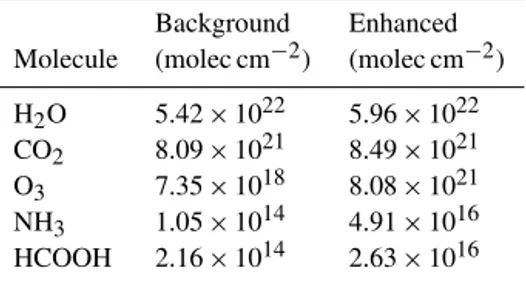
Table 1.Background and enhanced concentrations used in Fig. 1.
Background Enhanced Molecule (molec cm−2) (molec cm−2)
H2O 5.42×10²² 5.96×10²² CO2 8.09×10²¹ 8.49×10²¹ O3 7.35×10¹⁸ 8.08×10²¹ NH3 1.05×10¹⁴ 4.91×10¹⁶ HCOOH 2.16×10¹⁴ 2.63×10¹⁶
the HCOOH retrievals are only performed when the cloud optical depth is less than 1.0. Accurate and well-validated forward radiative transfer calculations are required for these detailed inversions. In this analysis we use OSS (Optimal Spectral Sampling)-TES, a rapid and accurate forward radi-ance model that employs an optimal spectral sampling tech-nique (Moncet et al., 2008). OSS-TES is built from the Line-By-Line Radiative Transfer Model (LBLRTM) (Clough et al., 2005), which has been well validated (e.g., Shephard et al., 2009; Mlawer et al., 2012; Alvarado et al., 2013). 2.2 TES HCOOH microwindows
The TES HCOOH retrieval uses the ν6-vibrational band at
1105 cm−1. Figure 1 shows simulated radiance signals for relevant atmospheric species in this relatively clean spectral window region. The background and enhanced concentra-tions used to calculate these spectral sensitivities are given in Table 1. Note that line intensities for this region from HI-TRAN (High Resolution Transmission) 2008 (Rothman et al., 2009), which are based on Vander Auwera et al. (2007), are up to two times greater than the HITRAN 2004 values (Rothman et al., 2005). This large change implies that earlier HCOOH measurements derived using HITRAN 2004 are too large by a similar amount.
Microwindows for the TES HCOOH retrieval are pre-sented in Table 2. While the HCOOH spectral feature in this region includes two side lobes, between 1192 and 1196 cm−1 and between 1112 and 1120 cm−1, we find that using the information in these lobes often leads to unstable retrievals when the HCOOH spectral signal is weak. The signal in these features tends to rise above the noise level only for large con-centrations of HCOOH.
2.3 Building a priori profiles and constraints
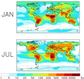
Simulated HCOOH mixing ratios from the GEOS-Chem CTM are shown in Fig. 2 for January and July 2004. Concen-trations are elevated over the continents and in the summer hemisphere, reflecting the predominantly terrestrial and pho-tochemical nature of the HCOOH sources in the model. The highest HCOOH levels are predicted over and downwind of regions with strong biogenic and pyrogenic emissions, such as the tropics and the southeastern United States. Only rarely
Figure 1.simulated spectra and residuals. Top panel:
TES-simulated spectra for background amounts of H2O, CO2, O3, NH3, and HCOOH (black line), and for enhanced amounts of each molecule (colored lines). Note that in several cases the perturbed spectra are obscured by the reference spectrum. Bottom panel: residuals computed as the reference spectrum minus the perturbed spectra. In both panels the blue triangles show the microwindows used for the formic acid retrieval. See Table 1 for background and enhanced amounts.
Table 2.Microwindows for TES HCOOH retrievals∗.
Index TES filter ν¯1(cm−1) ν¯2(cm−1) Purpose
1 1B2 1095.20 1095.32 Surface 2 1B2 1104.50 1105.64 HCOOH 3 1B2 1108.80 1109.06 Surface
∗ν
1andν2represent the left and right edges of the microwindows.
do the simulated surface concentrations exceed 2 ppbv (parts per billion by volume).
36
Figure 2.HCOOH in surface air as simulated by the GEOS-Chem
model for 2004.
36
Figure 3.HCOOH profiles simulated by GEOS-Chem over the
en-tire globe for 2004 binned by type (in grey). The mean profiles for each category are shown in color. See text for details.
(panels b and c). Further analysis of the retrieval showed that even the enhanced a priori profile led to very weak Jacobians which, when combined with a weaker HCOOH signal (1 K for the Australia cases versus 2 K for the ARCTAS case), did not allow the retrieval to reduce the residuals.
These results pointed to the need for a more enhanced a priori profile, corresponding to scenarios with much higher HCOOH concentrations than predicted by the CTM. This is consistent with the findings of Paulot et al. (2011), who found that atmospheric HCOOH tends to be underestimated by GEOS-Chem, at times by a factor of four or more. Air-craft measurements during the Intercontinental Transport Experiment-Phase B (INTEX-B) and Megacity Initiative: Local and Global Research Observations, (MILAGRO) cam-paigns also confirm the general tendency of GEOS-Chem to underestimate HCOOH, as shown by the average measured and modeled profiles for these campaigns (Fig. 5). There-fore, we concluded that the current state of understanding for HCOOH, as implemented in GEOS-Chem, does not pro-vide an adequate representation of the distribution and vari-ability of atmospheric HCOOH for deriving an appropriate a priori for the TES retrieval. We instead constructed an en-hanced a priori profile based on the IASI a priori (Razavi et al., 2011) and an analysis of HCOOH measurements from the
37
(c)
Figure 4.TES brightness temperature and retrieval residuals from an observation taken east of Australia (24.33◦S, 164.18◦W) on
2 February 2009 during the Black Saturday fire event. TES BT (top panel); residual before retrieval (second panel); residual after re-trieval with first a priori (third panel); residual after rere-trieval with final a priori (bottom panel).
MILAGRO campaign, and a clean a priori based on the MI-LAGRO data alone (Fig. 6). As we discuss in Sect. 3.3, clean profiles are in general below the TES detectability level. The diagonals of the covariance matrices used for constructing the constraint matrices were set to allow approximately 20 % variability for the clean cases and 50 % variability for the enhanced cases. Constraining the clean cases more tightly greatly reduces the chance of false positives, i.e., artificial detection of elevated HCOOH when there is little informa-tion from the observainforma-tions. These constraints will be refined as needed when more global information becomes available. The refined retrieval with the enhanced prior reduces the residuals to an acceptable level, as can be seen in the bottom panel of Fig. 4.
2.4 A priori selection
Figure 5.Mean HCOOH profiles from GEOS-Chem and aircraft
measurements during MILAGRO (left) and INTEX-B (right).
39
A
B Figure 6.Clean (blue) and enhanced (red) a priori profiles.
2011). However, unlike with IASI, in this case we are only using the BT difference to select an a priori profile for use in the subsequent full optimal estimation retrieval.
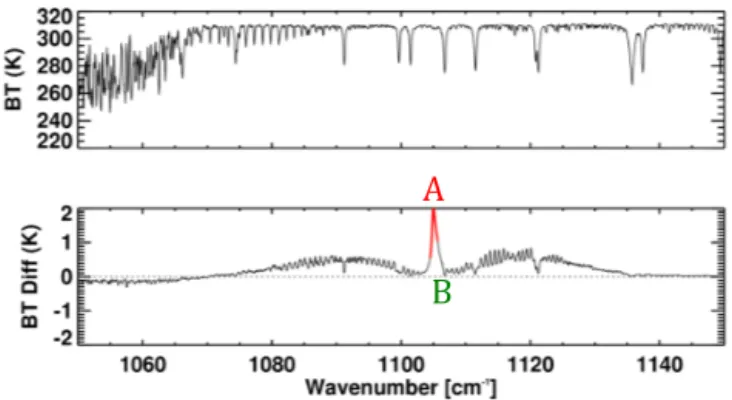
Figure 7 shows a simulated TES spectrum in the region where HCOOH is active along with the HCOOH signal, de-fined as the difference between forward model runs with and without HCOOH. The HCOOH peak and window sig-nals are calculated over 1105.04–1105.16 cm−1 (region A) and 1108.88–1109.06 cm−1(region B) respectively. The BT difference between the peak and window regions only pro-vides an estimate of the true HCOOH signal, which can be represented by the peak outlined in red from 1104.50 to 1105.64 cm−1. The estimated and true signals are corre-lated, but the relationship is not exact; different atmospheric conditions (e.g., water vapor amounts, surface conditions) lead to different ratios between the two parameters. In Fig. 8 we show a scatter plot of the SNR (the true HCOOH sig-nal divided by the expected noise) and the estimated sigsig-nal from the BT difference, obtained from 561 different forward model runs (see details in Sect. 3.2). There is a clear linear relationship between the two, with a correlation coefficient of 0.94. However, the degree of scatter illustrates that even in a simulation environment with no spectral noise and no
39
A
B
Figure 7.Simulated TES spectrum (top panel), and HCOOH
resid-ual (bottom panel).
retrieval errors in other species, the BT difference approach provides, at best, a first guess, which is its function in the TES HCOOH algorithm.
To select the a priori profile type to use in a particular TES HCOOH retrieval, the BT difference is first calculated at the spectral points listed above, and then transformed by the lin-ear relationship shown in Fig. 8 to provide an estimate of the SNR. If the absolute value of the SNR is greater than 2, then the enhanced a priori is used in the retrieval, other-wise the clean a priori is selected. In our discussion of the Black Saturday fire observations (Sect. 2.3), we noted that unless the a priori was significantly enhanced, the retrieval did not move towards a solution due to weak measurement sensitivity (small Jacobian values). While in many retrieval implementations the initial guess profile and the a priori are identical, this is not compulsory, and we find that in order to avoid null space issues (from weak Jacobians) in the TES HCOOH retrieval it is necessary to set the initial guess pro-file (but not the a priori propro-file itself) equal to the enhanced a priori in all cases.
3 TES HCOOH product
3.1 TES HCOOH retrieval characteristics
40
Figure 8.HCOOH SNR vs. estimated HCOOH signal (see text for
definitions) with linear fit parameters.
DOFS > 0.1, and of those, 54 % had DOFS > 0.5 and 24 % had DOFS > 0.8.
Since there are often one or fewer pieces of information in an individual measurement, the shape of the retrieved profile is strongly determined by the a priori profile. Retrieving col-umn (or partial colcol-umn) scale factors rather than vertically re-solved full profiles is a common strategy adopted where there is limited vertical information provided by the measurement. However, this implicitly assumes a profile shape and that the measurement is equally sensitive over all of the retrieved col-umn. Performing the HCOOH retrieval on a number of ver-tical profile levels has the advantage of capturing the region of maximum vertical sensitivity for each case, which varies from profile to profile depending on the atmospheric state.
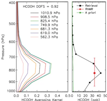
The fact that the retrieval is carried out on multiple verti-cal levels does not mean that the retrieved profile shape will adjust fully to the true profile in all cases. There is not suffi-cient information in the TES signal for this to occur. In par-ticular, the shape of the a priori profile employed in the TES retrieval is meant to reflect average conditions globally, and there are likely to be situations where HCOOH is enhanced aloft and the assumed shape thus does not accurately cap-ture the true vertical distribution. For example, the retrieved profile over the intense Australian Black Saturday fire shown in Fig. 9 peaks around 825 mbar, whereas the true peak in
41 1
Figure 9. Averaging kernel (left) and retrieved HCOOH profile
(right) from the TES spectrum shown in Fig. 4. The red circle shows the HCOOH RVMR and the red lines show the vertical extent over which the RVMR applies. The green line is the enhanced a priori profile.
this instance may be much higher in the atmosphere. This in an unavoidable issue when developing a general algorithm for all conditions; it is possible to create an a priori profile and a constraint matrix for specific situations, such as strong biomass burning plumes, which would return more accurate profiles, but we have not attempted this procedure here.
Given the low amount on information on the profile shape we use the Representative Volume Mixing Ratio (RVMR) (Payne et al., 2009; Shephard et al., 2011) method to map the retrieved profile VMRs to a subset of values that are more representative of the information content provided by TES; in the case of HCOOH this is typically one value. In other words, we aggregate the information provided by the satellite into a single metric that is minimally affected by the retrieval a priori:
RVMR=X
i
wixi, (1)
where for each leveli,wis the weighting function (in log
space) derived from the TES sensitivity as represented by the averaging kernel, andxis the log of the retrieved mixing
ratio. An example HCOOH RVMR is shown for the Black Saturday fires in Fig. 9 with the representative vertical range of the RVMR also indicated.
3.2 Results from simulated retrievals
42
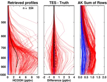
Figure 10. Simulated HCOOH retrievals over North America in July 2008. Colored curves indicate the a priori selection (blue: clean, red: enhanced). Left panel: retrieved profiles, with the mean retrieved profile in black. Middle panel: retrieved minus true pro-files. The solid line shows the mean bias, while the dashed line shows the standard deviation of the bias. Right panel: sum of the averaging kernel rows (SRAK) for each profile, with the mean in black. Means and standard deviations are not calculated for the sur-face level, since the height of this level ranges from above 1000 to less than 800 hPa.
where the “true” HCOOH profile is known. Simulated TES spectra were calculated from 561 TES Level 2 profiles with prescribed (“truth”) HCOOH profiles. These simulated HCOOH profiles were generated by applying a scale factor to either the clean or the enhanced a priori profile; the scale factor was calculated as the product of a value ranging from 10 at the surface to 1 above 300 mbar, and a random variable ranging between 0.5 and 1.0. The simulated radiances were computed for each profile by adding random noise that is typ-ical of the actual TES instrument noise in this spectral region (0.2–0.3 K). These simulated radiances were then provided as inputs to the retrieval algorithm. The a priori profile was selected according to the algorithm described in Sect. 2.4, and the initial guess was set to the enhanced a priori.
From the 561 spectra, we obtained 334 retrieved profiles with DOFS greater than 0.1, and the TES observational op-erator (defined in the Appendix) was then applied to the pre-scribed “true” HCOOH profiles. Retrievals with DOFS < 0.1 were excluded from the following analysis, since after apply-ing the TES operator the “true” and retrieved profiles in those cases would both be very similar to the a priori profile, which would bias the statistics.
Under these ideal simulated conditions where the truth is known, profile comparisons of the retrieved versus true pro-files in Fig. 10 show that the retrievals have a very small mean bias of−0.02 ppbv, with a standard deviation (SD) of
±0.37 ppbv at 825 hPa. More insight can be gained by bin-ning the retrieval bias and variance according to the a priori
Table 3.Simulated retrieval results at 825 hPa.
A priori Mean (ppbv) Bias (ppbv) SD (σ)
Clean 0.20 −0.005 (2.5 %) ±0.02 (10 %) Enhanced 5.02 −0.06 (1.2 %) ±0.61 (12 %)
43
Figure 11.Signal-to-noise ratio (SNR) vs. thermal contrast, color
coded by the maximum concentration of each profile.
type, as show in Table 3. Our simulated data set contains 100 cases with a clean a priori and 234 with an enhanced a priori. Note that the set of profiles classified as clean have retrievals that are significantly influenced by the a priori, and thus are expected to have a low bias; however, the retrievals over the enhanced profiles also have a very low bias (−0.06 ppbv) overall. These results demonstrate that the retrieval strategy performs well under ideal conditions where everything in the atmospheric state is known perfectly except HCOOH.
44
Figure 12.Thermal contrast, DOFS and maximum HCOOH value
vs. SNR for simulated retrievals.
3.3 TES HCOOH detection threshold
The minimum concentration threshold for detecting HCOOH from TES can be defined as the value where the SNR≡1; be-low that point the retrieved value is principally determined by the a priori. In Fig. 11 we show the SNR, defined in Sect. 2.4, as a function of the thermal contrast (the difference between the surface temperature and the air temperature at the first re-trieval level) for the set of simulated radiances discussed in the previous section. The points have been color-coded based on the maximum concentration of each “true” profile. The environmental conditions (e.g., surface properties, and atmo-spheric temperature profile) impact the infrared signal for a given HCOOH abundance. We see that profiles with a max-imum HCOOH concentration below roughly 0.5 ppbv are in general not detectable by TES, and thermal contrast plays a significant role in the strength of the HCOOH signal: even cases with high amounts (> 4.0 ppbv) may have a very low SNR with low thermal contrast, (less than 5 K) while fairly low-HCOOH cases (< 1 ppbv) may have a SNR over 1 if the thermal contrast is high enough (> 15 K). If we examine the statistics of the cases with SNR greater than 1, binned by SNR, (Fig. 12), we can refine the detection threshold. If we look at the results in the bin with lowest SNR values, and set as a detection threshold the maximum HCOOH in the 75– 90th percentile range, then we can state that the minimum detection threshold lies between 0.69 and 0.94 ppbv, though, as shown in Fig. 11, this requires significant thermal contrast. When using remote sensing data, one frequently needs to assess how much information for a given retrieval is being provided by the measurement, as opposed to the a priori as-sumption. In the case of the TES HCOOH measurements, the end user has no information on the SNR values; how-ever, the retrieval does provide the DOFS, which, as shown in the middle panel of Fig. 12, are fairly well correlated with
45
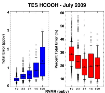
Figure 13.HCOOH RVMR-estimated errors for a TES Global
Sur-vey from July 2009, binned by RVMR value: absolute error (left panel), percent error (right panel).
the signal strength, though they tend asymptotically to 1.0 for high SNR. When the HCOOH signal is less than the noise level (SNR < 1) the DOFS are generally less than 0.5. This implies that the retrieved profile will be very similar to the prior or, equivalently, that the retrieval has added little to the estimate of the true state. There are a number of cir-cumstances that can lead to retrieved HCOOH amounts with low DOFS, including clean conditions with low concentra-tions of HCOOH, cold scenes with limited infrared radiance, thicker cloud, and cases with little thermal contrast between the surface and the atmospheric layers containing HCOOH, as shown in Fig. 11. Thus, the DOFS can be used as a rough criteria for accepting or rejecting retrievals in an analysis. 3.4 TES HCOOH error estimates
Error estimates derive directly from optimal estimation re-trievals (Rodgers 2000; Worden et al., 2004); see Eq. (A3) in the Appendix. These retrieval errors can then be mapped into the RVMR space via the same weighting matrix (W )used to
calculate the RVMR itself (Cady-Pereira et al., 2012):
E=WH−1WT, (2)
whereE is the error in the RVMR, andHis the Hessian, computed as
H=S−a1+KTS−n1K (3)
(refer to the Appendix for definitions ofSa,K, andSn).
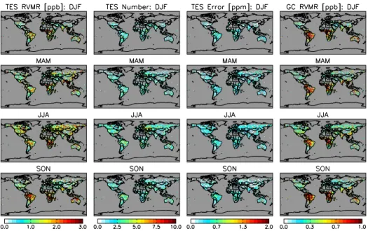
Figure 14.2009 HCOOH: TES RVMR (column 1), number of TES observations (column 2), TES estimated error (column 3) and
GEOS-Chem with TES operator applied (column 4).
increasing HCOOH; while there are some large outliers in the relative error, especially when HCOOH is low, the esti-mated relative errors are mostly in the 10–35 % range.
For the error analysis performed here we have not ex-plicitly taken into consideration any systematic components (i.e., the last term in Appendix Eq. A3). One potential source of systematic error in the retrieval is uncertainty in the spectroscopic parameters; for example, line intensity er-rors would yield directly proportional erer-rors in the retrieved HCOOH concentrations. HCOOH spectroscopic parameters used in these retrievals are from the HITRAN 2008 database (Rothman et al., 2009), with estimated uncertainties in the line intensities of∼7 % (Vander Auwera et al., 2007). Since this error is small relative to the overall estimated error for the TES HCOOH measurement it is ignored for this initial analy-sis, but could be important for future retrieval improvements. Another potential source of systematic error is the propaga-tion of errors from other retrieved parameters (i.e., temper-ature, water vapor retrievals, surface temperature and emis-sivity) onto the HCOOH retrieval. We have not taken into ac-count these systematic or cross-state errors in this initial anal-ysis. Our assumption is that these errors are small relative to the estimated random errors, as the retrieval microwindow is narrow and the first step of the retrieval (i.e., for surface tem-perature and emissivity) will have reduced the background radiance residuals to (or close to) the noise level. Conclusive characterization of the full uncertainty (i.e., both systematic and random components) in the TES HCOOH measurements requires comparisons with independent data; such compar-isons will be presented in a subsequent paper.
4 Results from TES global surveys
Figure 14 shows the global and seasonal distribution of at-mospheric HCOOH as measured by TES (2009 Global Sur-veys) and as simulated for the same year by GEOS-Chem. Due to the low SNR over the oceans (from the expected low HCOOH concentrations and reduced thermal contrast), we include here only retrievals over land. There is also a paucity of successful HCOOH observations over desert regions such as North Africa and the Arabian Peninsula, due to retrieval challenges arising from the strong silicate spectral feature in surface emissivity for these areas.
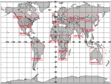
Figure 15.Regions used for aggregating data for Figs. 16 and 17.
55 Tg globally in 2009, including 47 Tg from photochemical production, 4.2 Tg from direct biogenic emissions (including soils), 1.5 Tg from direct fire emissions, and 2.6 Tg from an-thropogenic and agricultural sources.
The global, average atmospheric lifetime of HCOOH in the model is 3.3 days, with sinks due to dry deposition (ac-counting for 39 % of the total sink in 2009) computed based on a standard resistance-in-series scheme (Wesely, 1989), wet deposition as described by Amos et al. (2012) (38 %), and photochemical oxidation by OH (23 %).
For each successful TES HCOOH retrieval over land with DOFS > 0.1 we sample GEOS-Chem at the time and location of the measurement, and apply the TES observational oper-ator to the model profile. The first step ensures that model grid boxes not sampled by TES are excluded from the analy-sis, while the last step provides a self-consistent comparison that accounts for the vertical sensitivity of the satellite mea-surement. We then compute RVMR values for both TES and GEOS-Chem as described in Sect. 3.1; these are then aver-aged seasonally and onto the 2◦×2
.5◦GEOS-Chem model
grid. The number of valid retrievals and the mean error in each box are also calculated.
We see in Fig. 14 that the broad spatial distribution of HCOOH simulated by GEOS-Chem has some similarities to that observed by TES. For example, in both cases there are elevated HCOOH concentrations in the tropics and in the Northern Hemisphere during summer, and biomass burning seasons are obvious in Africa and South America. However, the model RVMRs are persistently low compared to TES, typically by a factor of two or more. Since the number of TES observations in any given model grid box is usually low (Fig. 14, second column), and the errors are a signifi-cant fraction of the retrieved value (Fig. 14, third column), we have aggregated the TES and GEOS-Chem results by re-gions (Fig. 15), in order to obtain more meaningful statistics (Figs. 16 and 17, respectively).
48
Figure 16.Statistics of the TES HCOOH RVMR values in Fig. 14
for each region in Fig. 15. Boxes indicate the 25th and 75th per-centiles, the line and diamond correspond to the median and the mean, the whiskers indicate the 10th and 90th percentiles, and the outliers are represented by the circles.
Figure 17.As in Fig. 16, but for the GEOS-Chem RVMR values in
Fig. 14 and different vertical scale.
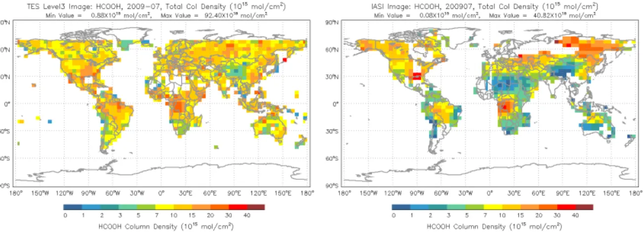
1
Figure 18.HCOOH total columns for July 2009 for TES (left) and IASI (right).
The aggregated results confirm the similarity in the sea-sonal cycle in most regions, most notably over Australia, South America, Mexico, northern Central Africa and south-ern Africa, but also highlight the much weaker seasonal am-plitude. The most pronounced model-measurement discrep-ancies seen in Fig. 14 occur in summertime and season-ally over biomass burning regions (e.g., Amazonia, Africa, northern Australia). The model concentrations are also some-what elevated during those times, but nonetheless exhibit a dramatic low bias compared to TES. This suggests a sig-nificant missing source of HCOOH from biogenic as well as pyrogenic sources, either through direct emission or sec-ondary production from co-emitted precursors (Stavrakou et al., 2012; Paulot et al., 2011). The TES data thus corrobo-rate other recent studies based on aircraft, surface FTS, and satellite measurements that have pointed to large-scale miss-ing sources of atmospheric HCOOH (Stavrakou et al., 2012; Paulot et al., 2011). That these HCOOH measurements are obtained from very different sensors and a variety of methods strengthens the argument for these missing sources. As an il-lustration of the general agreement between TES and IASI HCOOH we have calculated the mean TES total columns on the 4×5 degree grid used by the IASI team for July 2009 (Fig. 18). Even though the total column obtained for each sensor is influenced by the a priori profile adopted for that sensor, regions with enhanced HCOOH present values in the same range: central Brazil (15–20 molec cm−2), eastern sub-Saharan Africa (30–40 molec cm−2), the eastern US (20– 40 molec cm−2) and eastern Siberia (10–30 molec cm−2), though some of the IASI values are higher in this region. We are working on validating the TES HCOOH product (Chaliyakunnel et al., 2014) and will carry out a more ex-tensive and quantitative comparison between TES and IASI HCOOH. We will also apply the TES data to investigate the missing HCOOH sources.
5 Conclusions
Advances in infrared satellite observations are providing new global information on atmospheric species with relatively weak spectral signals, and have potential to yield valuable insights on processes driving tropospheric chemistry and air quality. In this paper, we presented the TES HCOOH re-trieval, including the overall strategy, algorithm specifics, and error characterization.
Simulated retrievals show that because of its relatively weak spectral signature, measurements of HCOOH from TES in general have at most 1.0 DOFS, and usually less. The TES HCOOH retrieval is most sensitive in the mid-to-lower troposphere (850–600 hPa), with a vertical resolution of∼2 km. The minimum detection limit for TES HCOOH is a peak profile value of∼0.7 ppbv under conditions with
strong thermal contrast (∼10 K), with the detection limit
in-creasing as thermal contrast decreases. The ensemble of sim-ulated HCOOH retrievals also show that under ideal condi-tions, and in the absence of systematic errors in the spectro-scopic parameters or in other retrieved quantities, the TES HCOOH retrievals are unbiased with a standard deviation of
x xa A( a) G GKb( a), (A1)
wherexˆ,xa, andxare the retrieved, a priori, and the “true”
state vectors respectively. The gain matrix, G, maps from spectral radiance space into retrieval parameter space, and the vector nrepresents the noise on the measured spectral
radiances. The vectorbrepresents the true state for other
pa-rameters that are not measured in the HCOOH retrieval it-self, but that may nonetheless impact the HCOOH retrieval results (e.g., concentrations of interfering gases, calibration, etc.). The vectorba contains the corresponding a priori
val-ues, andK=∂L/∂bis a Jacobian describing the dependence
of the forward model radiancesLon the parameters in vector
b.
The averaging kernel, A, describes the sensitivity of the retrieval to the true state:
A=∂x˙ˆ
∂x =(K
TS−1
n K+S−a1)−1KTS−n1K=GK, (A2) whereSnis the instrument noise covariance matrix, andSais the a priori constraint matrix for the retrieval. The Jacobian, K, is the sensitivity of the forward model radiances to the state vector of the parameters being retrieved (in this case, HCOOH mixing ratios),K=∂L/∂x.
Sx=(Axx−I)Sa(Axx−I) +GSnG
+GKbSb(GKb)T, (A3)
whereSbis the expected covariance of the nonretrieved
pa-rameters. The total error for a retrieved profile is expressed as the sum of (i) the smoothing errors (first term on the right-hand side), i.e., the uncertainty due to unresolved fine struc-ture in the profile; (ii) the measurement errors (second term) originating from random noise in the spectrum; and (iii) the systematic errors (last term) due to uncertainties in the non-retrieved forward model parameters, some of which are con-stant and some of which change from retrieval to retrieval (Worden et al., 2004).
Acknowledgements. We thank Tom Connor, Alan Lipton, Jean-Luc Moncet, and Gennady Uymin of AER for building an OSS version for TES. We also thank Paul Wennberg and the MILAGRO and INTEX-B teams for providing the data from these campaigns and the IASI team at the Universite Libre de Bruxelles for providing the IASI HCOOH data. Research at JPL was supported under contract to the National Aeronautics and Space Administration (NASA). Research at AER was supported under contract to NASA and the University of Minnesota. Work at UMN was supported by NSF through the Atmospheric Chemistry Program (grant no. AGS-1148951), by NASA through the Atmospheric Chemistry Modeling and Analysis Program (grant no. NNX10AG65G), and by the University of Minnesota Supercomputing Institute. The TES HCOOH product is available at http://tes.jpl.nasa.gov/data/.
Edited by: E. C. Apel
References
Alvarado, M. J., Cady-Pereira, K. E., Xiao, Y., Millet, D. B., and Payne, V. H.: Emission Ratios for Ammonia and Formic acid and Observations of Peroxy Acetyl Nitrate (PAN) and Ethy-lene in Biomass Burning Smoke as Seen by the Tropospheric Emission Spectrometer (TES), Atmosphere, ISSN 2073-4433, doi:10.3390/atmos2040633, 2011.
Alvarado, M. J., Payne, V. H., Mlawer, E. J., Uymin, G., Shephard, M. W., Cady-Pereira, K. E., Delamere, J. S., and Moncet, J.-L.: Performance of the Line-By-Line Radiative Transfer Model (LBLRTM) for temperature, water vapor, and trace gas retrievals: recent updates evaluated with IASI case studies, Atmos. Chem. Phys., 13, 6687–6711, doi:10.5194/acp-13-6687-2013, 2013. Amos, H. M., Jacob, D. J., Holmes, C. D., Fisher, J. A., Wang,
Q., Yantosca, R. M., Corbitt, E. S., Galarneau, E., Rutter, A. P., Gustin, M. S., Steffen, A., Schauer, J. J., Graydon, J. A., Louis, V. L. St., Talbot, R. W., Edgerton, E. S., Zhang, Y., and Sunder-land, E. M.: Gas-particle partitioning of atmospheric Hg(II) and its effect on global mercury deposition, Atmos. Chem. Phys., 12, 591–603, doi:10.5194/acp-12-591-2012, 2012.
Andreae, M. O., Andreae, T. W., Talbot, R. W., and Harriss, R. C.: Formic and acetic acid over the central Amazon re-gion, Brazil. I. Dry season, J. Geophys. Res., 93, 1616–1624, doi:10.1029/JD093iD02p01616, 1988.
Andrews, D. U., Heazlewood, B. R., Maccarone, A. T., Conroy, T., Payne, R. J., Jordan, M. J. T., and Kable, S. H.: Photo-tautomerization of Acetaldehyde to Vinyl Alcohol: A Potential Route to Tropospheric Acids Science, 337, 1203–1206, 2012. Archibald, A. T., McGillen, M. R., Taatjes, C. A., Percival,
C. J., and Shallcross, D. E.: Atmospheric Transformation of Enols: A Potential Secondary Source of Carboxylic Acids in the Urban Troposphere, Geophys. Res. Lett., 34, L21801, doi:10.1029/2007GL031032, 2007.
Beer, R., Glavich, T. A., and Rider, D. M.: Tropospheric emission spectrometer for the Earth Observing System’s Aura satellite, Appl. Optics, 40, 2356–2367, 2001.
Bohn, B., Siese, M., and Zetzschn, C.: Kinetics of the OH+C2H2 reaction in the presence of O2, J. Chem. Soc., Faraday Trans., 92, 1459–1466, 1996.
Bowman, K. W., Rodgers, C. D., Sund-Kulawik, S., Worden, J., Sarkissian, E., Osterman, G., Steck, T., Luo, M.,
Elder-ing, A., Shephard, M. W., Worden, H., Clough, S. A., Brown, P. D., Rinsland, C. P., Lampel, M., Gunson, M., and Beer, R.: Tropospheric emission spectrometer: Retrieval method and error analysis, IEEE Geosci. Remote Sens., 44, 1297–1307, doi:10.1109/TGRS.2006.871234, 2006.
Cady-Pereira, K. E., Shephard, M. W., Millet, D. B., Luo, M., Wells, K. C., Xiao, Y., Payne, V. H., and Worden, J.: Methanol from TES global observations: retrieval algorithm and seasonal and spatial variability, Atmos. Chem. Phys., 12, 8189–8203, doi:10.5194/acp-12-8189-2012, 2012.
Chaliyakunnel, S., Dylan, B., Millet, K. C., Wells, K. E., Cady-Pereira, M. W., Shephard, M., Luo, M., and Paulot, F.: Global tropospheric formic acid measurements from the TES satellite sensor: retrieval evaluation and the importance of biogenic and pyrogenic sources, in preparation, 2014.
Clough, S. A., Shephard, M. W., Mlawer, E. J., Delamere, J. S., Iacono, M. J., Cady-Pereira, K., Boukabara, S., and Brown, R. D.: Atmospheric radiative transfer modeling: a summary of the AER codes, J. Quant. Spectrosc. Ra., 91, 233–244, 2005. Clubb, A. E., Jordan, M. J. T., Kable, S. H., and Osborn, D. L.:
Pho-totautomerization of Acetaldehyde to Vinyl Alcohol: A Primary Process in UV-Irradiated Acetaldehyde from 295 to 335 nm, J. Phys. Chem. Lett., 3, 3522–3526, 2012.
Coheur, P.-F., Clarisse, L., Turquety, S., Hurtmans, D., and Cler-baux, C.: IASI measurements of reactive trace species in biomass burning plumes, Atmos. Chem. Phys., 9, 5655–5667, doi:10.5194/acp-9-5655-2009, 2009.
Connor, T. C., Shephard, M. W., Payne, V. H., Cady-Pereira, K. E., Kulawik, S. S., Luo, M., Osterman, G., and Lampel, M.: Long-term stability of TES satellite radiance measurements, At-mos. Meas. Tech., 4, 1481–1490, doi:10.5194/amt-4-1481-2011, 2011.
da Silva, G.: Carboxylic acid catalyzed keto-enol tautomerizations in the gas phase, Angew. Chem., 122, 7685–7687, 2010. Goode, J. G., Yokelson, R. J., Ward, D. E., Susott, R. A.,
Bab-bitt, R. E., Davies, M. A., and Hao, W. M.: Measurements of excess O3, CO2, CO, CH4, C2H4, C2H2, HCN, NO, NH3, HCOOH, CH3COOH, HCHO, and CH3OH in 1997 Alaskan biomass burning plumes by airborne fouriertransform infrared spectroscopy (AFTIR), J. Geophys. Res., 105, 22147–22166, 2000.
Grutter, M., Glatthor, N., Stiller, G. P., Fischer, H., Grabowski, U., Höpfner, M., Kellmann, S., Linden, A., and von Clarmann, T.: Global distribution and variability of formic acid as ob-served by MIPAS-ENVISAT, J. Geophys. Res., 115, D10303, doi:10.1029/2009JD012980, 2010.
Guenther, A. B., Jiang, X., Heald, C. L., Sakulyanontvittaya, T., Duhl, T., Emmons, L. K., and Wang, X.: The Model of Emissions of Gases and Aerosols from Nature version 2.1 (MEGAN2.1): an extended and updated framework for modeling biogenic emis-sions, Geosci. Model Dev., 5, 1471–1492, doi:10.5194/gmd-5-1471-2012, 2012.
Hatch, C. D., Gough, R. V., and Tolbert, M. A.: Heterogeneous up-take of the C1 to C4 organic acids on a swelling clay mineral, At-mos. Chem. Phys., 7, 4445–4458, doi:10.5194/acp-7-4445-2007, 2007.
Artaxo, P., Alves, E., Kesselmeier, J., Taylor, T., Saleska, S., and Huxman, T.: Ecosystem-scale compensation points of formic and acetic acid in the central Amazon, Biogeosciences, 8, 3709– 3720, doi:10.5194/bg-8-3709-2011, 2011.
JPL: TES Level 2 Data User’s Guide, edited by: Osterman, G., 2006.
Karton, A.: Inorganic acid-catalyzed tautomerization of vinyl alco-hol to acetaldehyde, Chem. Phys. Lett., 592, 330–333, 2014. Kawamura, K., Ng, L. L., and Kaplan, I. R.: Determination of
or-ganic acids (C1–C10) in the atmosphere, motor exhausts, and engine oils, Environ. Sci. Technol., 19, 1082–1086, 1985, 1985. Keene, W. C. and Galloway, J. N.: The biogeochemical cycling
of-formic and acetic acids through the troposphere: An overview of current understanding, Tellus B, 40, 322–334, 1988.
Kesselmeier, J., Bode, K., Gerlach, C., and Jork, E. M.: Exchange of atmospheric formic and acetic acids with trees and crop plants under controlled chamber and purified air conditions, Atmos. En-viron., 32, 1765–1775, 1998.
Kuhn, U., Rottenberger, S., Biesenthal, T., Ammann, C., Wolf, A., Schebeske, G., Oliva, S. T., Tavares, T. M., and Kesselmeier, J.: Exchange of short-chain monocarboxylic acids by vegetation at a remote tropical forest site in Amazonia, J. Geophys. Res., 107, 8069, doi:10.1029/2000JD000303, 2002.
Kulawik, S. S., Worden, J., Eldering, A., Bowman, K., Gunson, M., Osterman, G. B., Zhang, L., Clough, S., Shephard, M. W., and Beer, R.: Implementation of cloud retrievals for Tropospheric Emission Spectrometer (TES) atmospheric retrievals: part 1. De-scription and characterization of errors on trace gas retrievals, J. Geophys. Res., 111, D24204, doi:10.1029/2005JD006733, 2006. Lawrence, D. M., Oleson, K. W., Flanner, M. G., Thornton, P. E., Swenson, S. C., Lawrence, P. J., Zeng, X., Yang, Z.-L., Levis, S., Sakaguchi, K., Bonan, G. B., and Slater, A. G.: Parameterization improvements and functional and structural advances in version 4 of the Community Land Model, J. Adv. Model. Earth Sys., 3, M03001, doi:10.1029/2011MS000045, 2011.
Lee, A., Goldstein, A. H., Kroll, J. H., Ng, N. L., Varut-bangkul, V., Flagan, R. C., and Seinfeld, J. H.: Gas-phase products and secondary aerosol yields from the photooxida-tion of 16 different terpenes, J. Geophys. Res., 111, D17305, doi:10.1029/2006JD007050, 2006.
Mlawer, E. J., Payne, V. H., Moncet, J.-L., Delamere, J. S., Al-varado, M. J., and Tobin, D. C.: Development and recent eval-uation of the MT_CKD model of continuum absorption, Philos. T. Roy. Soc. A, 370, 1–37, doi:10.1098/rsta.2011.0295, 2012.
limited degrees of freedom for signal: Application to methane from the Tropospheric Emission Spectrometer, J. Geophys. Res., 114, D10307, doi:10.1029/2008JD010155, 2009.
Payne, V. H., Alvarado, M. J., Cady-Pereira, K. E., Worden, J. R., Kulawik, S. S., and Fischer, E. V.: Satellite observa-tions of peroxyacetyl nitrate from the Aura Tropospheric Emis-sion Spectrometer, Atmos. Meas. Tech. Discuss., 7, 5347–5379, doi:10.5194/amtd-7-5347-2014, 2014.
Paulot, F., Wunch, D., Crounse, J. D., Toon, G. C., Millet, D. B., DeCarlo, P. F., Vigouroux, C., Deutscher, N. M., González Abad, G., Notholt, J., Warneke, T., Hannigan, J. W., Warneke, C., de Gouw, J. A., Dunlea, E. J., De Mazière, M., Griffith, D. W. T., Bernath, P., Jimenez, J. L., and Wennberg, P. O.: Im-portance of secondary sources in the atmospheric budgets of formic and acetic acids, Atmos. Chem. Phys., 11, 1989–2013, doi:10.5194/acp-11-1989-2011, 2011.
Pinder, R. W., Walker, J. T., Bash, J. O., Cady-Pereira, K. E., Henze, D. K., Luo, M., and Shephard, M. W.: Quantifying spa-tial and temporal variability in atmospheric ammonia with in situ and space-based observations, Geophys. Res. Lett., 38, L04802, doi:10.1029/2010GL046146, 2011.
Razavi, A., Karagulian, F., Clarisse, L., Hurtmans, D., Coheur, P. F., Clerbaux, C., Müller, J. F., and Stavrakou, T.: Global distribu-tions of methanol and formic acid retrieved for the first time from the IASI/MetOp thermal infrared sounder, Atmos. Chem. Phys., 11, 857–872, doi:10.5194/acp-11-857-2011, 2011.
Rinsland, C. P., Boone, C. D., Bernath, P. F., Mahieu, E., Zander, R., Dufour, G., Clerbaux, C., Turquety, S., Chiou, L., Mc-Connell, J. C., Neary, L., and Kaminski, J. W.: Atmospheric Chem-istry Experiment austral spring 2004 and 2005 Southern Hemi-sphere tropical-mid-latitude upper tropospheric measurements, Geophys. Res. Lett, 33, L23804, doi:10.1029/2006GL027128, 2006.
Rinsland, C. P., Dufour, G., Boone, C. D., Bernath, P. F., Chiou, L., Coheur, P.-F., Turquety, S., and Clerbaux, C.: Satellite boreal measurements over Alaska and Canada during June– July 2004: Simultaneous measurements of upper tropospheric CO,C2H6, HCN, CH3Cl, CH4, C2H2, CH3OH, HCOOH, OCS, and SF6 mixing ratios, Global Biogeochem. Cy., 21, B3008, doi:10.1029/2006GB002795, 2007.
Rodgers, C. D.: Inverse methods for atmospheric Sounding: Theory and Practice, World Sci., Hackensack, N. J., 2000.
Mandin, J.-Y., Massie, S. T., Orphal, J., Perrin, A., Rinsland, C. P., Smith, M. A. H., Tennyson, J., Tolchenov, R. N., Toth, R. A., Vander Auwera, J., Varanasi, P., and Wagner, G.: The HITRAN 2004 molecular spectroscopic database, J. Quant. Spectrosc. Ra., 96, 139–204, 2005.
Rothman, L. S., Gordon, I. E., Barbe, A., Benner, D. C., Bernath, P. F., Birk, M., Boudon, V., Brown, L. R., Campargue, A., Cham-pion, J.-P., Chance, K., Coudert, L. H., Dana, V., Devi, V. M., Fally, S., Flaud, J.-M., Gamache, R. R., Goldman, A., Jacque-mart, D., Kleiner, I., Lacome, N., Lafferty, W. J., Mandin, J.-Y., Massie, S. T., Mikhailenko, S. N., Miller, C. E., Moazzen-Ahmadi, N., Naumenko, O. V., Nikitin, A. V., Orphal, J., Perevalov, V. I., Perrin, A., Predoi-Cross, A., Rinsland, C. P., Rot-ger, M., Šimecková, M., Smith, M. A. H., Sung, K., Tashkun, S. A., Tennyson, J., Toth, R. A., Vandaele, A. C., and Vander Auw-era, J.: The HITRAN 2008 molecular spectroscopic database, J. Quant. Spectrosc. Ra., 110, 533–572, 2009.
Sanhueza, E. and Andreae, M. O.: Emission of formic and acetic acids from tropical savanna soils, Geophys. Res. Lett., 18, 1707– 1710, 1991.
Shephard, M. W., Worden, H. M., Cady-Pereira, K. E., Lampel, M., Luo, M., Bowman, K. W., Sarkissian, E., Beer, R., Rider, D. M., Tobin, D. C., Revercomb, H. E., Fisher, B. M., Tremblay, D., Clough, S. A., Osterman, G. B., and Gunson, M.: Tropospheric Emission Spectrometer Spectral Radiance Comparisons, J. Geo-phys. Res., 113, D15S05, doi:10.1029/2007JD008856, 2008. Shephard, M. W., Clough, S. A., Payne, V. H., Smith, W. L., Kireev,
S., and Cady-Pereira, K. E.: Performance of the line-by-line ra-diative transfer model (LBLRTM) for temperature and species retrievals: IASI case studies from JAIVEx, Atmos. Chem. Phys., 9, 7397–7417, doi:10.5194/acp-9-7397-2009, 2009.
Shephard, M. W., Cady-Pereira, K. E., Luo, M., Henze, D. K., Pin-der, R. W., Walker, J. T., Rinsland, C. P., Bash, J. O., Zhu, L., Payne, V. H., and Clarisse, L.: TES ammonia retrieval strat-egy and global observations of the spatial and seasonal vari-ability of ammonia, Atmos. Chem. Phys., 11, 10743–10763, doi:10.5194/acp-11-10743-2011, 2011.
So, S., Wille, U., and da Silva, G.: Atmospheric chemistry of enols: A theoretical study of the vinayl alcohol + OH + O2 reaction mechanism, Environ. Sci. Technol., 48, 6694–6701, doi:10.1021/es500319q, 2014.
Stavrakou, T., Müller, J.-F., Peeters, J., Razavi, A., Clarisse, L., Clerbaux, C., Coheur, P.-F., Hurtmans, D., De Mazière, M., Vigouroux, C., Deutscher, N. M., Griffith, D. W. T., Jones, N., and Paton-Walsh, C.: Satellite evidence for a large source of formic acid from boreal and tropical forests, Nat. Geosci., 5, 26– 30, doi:10.1038/ngeo1354, 2012.
Talbot, R. W., Beecher, K. M., Harriss, R. C., and Cofer, W. R.: Atmospheric geochemistry of formic and acetic acids at a mid-latitude temperate site, J. Geophys. Res., 93, 1638–1652, 1988. Vander Auwera, J., Didriche, K., Perrin, A., and Keller, F.:
Abso-lute line intensities for formic acid and dissociation constant of the Dimer, J. Chem. Phys., 126, 124311, doi:10.1063/1.2712439, 2007.
van der Werf, G. R., Randerson, J. T., Giglio, L., Collatz, G. J., Mu, M., Kasibhatla, P. S., Morton, D. C., DeFries, R. S., Jin, Y., and van Leeuwen, T. T.: Global fire emissions and the contribution of deforestation, savanna, forest, agricultural, and peat fires (1997– 2009), Atmos. Chem. Phys., 10, 11707–11735, doi:10.5194/acp-10-11707-2010, 2010.
Wells, K. C., Millet, D. B., Hu, L., Cady-Pereira, K. E., Xiao, Y., Shephard, M. W., Clerbaux, C. L., Clarisse, L., Coheur, P.-F., Apel, E. C., de Gouw, J., Warneke, C., Singh, H. B., Gold-stein, A. H., and Sive, B. C.: Tropospheric methanol observations from space: retrieval evaluation and constraints on the seasonal-ity of biogenic emissions, Atmos. Chem. Phys., 12, 5897–5912, doi:10.5194/acp-12-5897-2012, 2012.
Wells, K. C., Millet, D. B., Cady-Pereira, K. E., Shephard, M. W., Henze, D. K., Bousserez, N., Apel, E. C., de Gouw, J., Warneke, C., and Singh, H. B.: Quantifying global terrestrial methanol emissions using observations from the TES satellite sensor, At-mos. Chem. Phys., 14, 2555–2570, doi:10.5194/acp-14-2555-2014, 2014.
Wesely, M. L.: Parameterization of surface resistance to gaseous dry deposition in regional-scale numerical models, Atmos. Environ., 23, 1293–1304, 1989.
Worden, J., Kulawik, S. S., Shephard, M. W., Clough, S. A., Worden, H., Bowman, K., and Goldman, A.: Predicted er-rors of tropospheric emission spectrometer nadir retrievals from spectral window selection, J. Geophys. Res., 109, D09308, doi:10.1029/2004JD004522, 2004.